Deep Learning Notes - 8: GANs, Normalizing Flows, Autoencoders, and Diffusion Models
Deep Learning Notes - 8, covering four major generative models: GANs, normalizing flows, autoencoders and variational autoencoders (VAE), and diffusion models. Corresponds to Chapters 17-20 of "Deep Learning: Foundations and Concepts".
Part 8/8 of the series (final) ← Previous | Glossary
It is recommended to read Parts 1-7 first, especially Part 7 on sampling methods and latent variable models. This part covers four generative models: GANs, normalizing flows, autoencoders, and diffusion models.
Chapter 17 Generative Adversarial Networks (GAN)
You can check out kaggle - I’m also a painter↗ (you
Adversarial Training
In plain words: The core idea of a GAN can be understood through the analogy of a “forger vs. authenticator.” The Generator is like someone forging paintings; its goal is to produce fakes that are indistinguishable from the real thing. The Discriminator is like an appraiser; its goal is to tell which paintings are real and which are fakes. The two continuously play against each other—the forger’s skill keeps improving, and the appraiser’s eye keeps sharpening—until eventually the forger can produce works that pass as genuine.
The goal of a generative model is to learn the probability distribution (i.e., the data’s “generative law”) from which samples in the training dataset are drawn. Once the model has learned this distribution, it can generate new samples similar to the training data.
- Parametric Model: We introduce a generative model with learnable parameters , where is a vector in the data space (such as pixel values of an image) and is the model’s learnable parameter.
- Conditional Generative Model: Sometimes we want to generate samples of a specific type, such as generating an image of a cat. This can be achieved by introducing a condition variable , turning the model into . can be a class label (such as “cat” or “dog”) or a more complex description.
The first class of generative models discussed in this chapter is the Nonlinear Latent Variable Model. Its core idea is to map a simple low-dimensional latent distribution (the distribution followed by the latent variable ) to a complex high-dimensional data distribution through a nonlinear transformation.
Remember the latent variable model from Part 7? GANs use the same framework: a simple latent variable is transformed by a neural network into a complex data sample .
- Latent Space: We introduce a low-dimensional latent variable that follows a simple prior distribution , typically chosen to be a standard normal distribution:
- Generator Network: We define a nonlinear function implemented by a deep neural network, where are the network’s weight parameters. This network is called the Generator.
- Implicit Distribution: Together, the generator network and the prior distribution implicitly define a distribution over the data space. We cannot write down the analytical form of , but we can generate samples that follow by sampling from and computing .
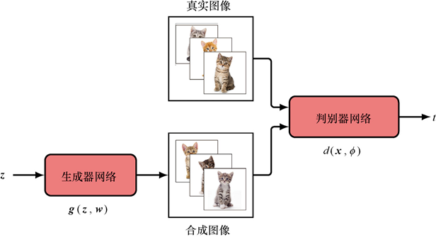
Adversarial network: the generator produces fake images from latent variable z, and the discriminator judges whether the input is real or fake
The figure above shows the overall architecture of a GAN:
- Left: a “Latent Variable” is fed into the “Generator” network , producing “Synthetic Images” .
- Middle: a “Discriminator” network . The discriminator receives two types of input: “Real Images” from the training set and the synthetic images from the generator.
- The discriminator outputs a scalar , representing the probability that the input image is a real image.
Adversarial Training
Adversarial training is the core mechanism of a GAN. It introduces a second network—the Discriminator—which plays a game against the generator.
- Discriminator Network: This is a classification neural network with parameters . Its task is to distinguish whether an input image comes from the real dataset or is a synthetic image produced by the generator. The discriminator’s output is a scalar between 0 and 1, representing the probability that the input image is real.
- The Game Process (imagine a showdown between a forger and an appraiser):
- Generator’s objective: Maximize the discriminator’s error rate. It wants the generated image to “fool” the discriminator into thinking it is a real image, i.e., .
- Discriminator’s objective: Minimize its own error rate. It wants to accurately distinguish real images from synthetic ones: for a real image , it outputs ; for a synthetic image , it outputs .
Mathematical form of the adversarial loss function (minimax game)
This game can be formalized as a minimax game:
where:
- The first term is the discriminator’s log-likelihood on real data (the discriminator wants to maximize this term).
- The second term is the discriminator’s log-likelihood on synthetic data. The discriminator wants to maximize this term, while the generator wants to minimize it.
In short: the discriminator wants this value to be as large as possible, and the generator wants it to be as small as possible.
Training Process
You may ask: how do the forger and the appraiser “train together”? The answer is alternating training—first fix one and train the other, then swap.
- Training the discriminator (with the generator fixed):
- Sample a batch of real samples from the real dataset.
- Sample a batch of from the latent distribution , and obtain a batch of synthetic samples through the generator.
- Compute the discriminator’s loss , so that it learns to tell real from fake:
- Use gradient descent to update the discriminator parameters to minimize .
- Training the generator (with the discriminator fixed):
- Sample a batch of from the latent distribution .
- Obtain synthetic samples through the generator.
- Compute the generator’s loss .
Why is the generator's loss function written differently?
The original generator loss has a problem in the early stages of training: when the generator is very weak and the discriminator easily tells real from fake, , so , and the gradient is nearly zero—the generator “cannot learn.”
Therefore, in practice an alternative objective is used: This objective maximizes the probability that the discriminator considers the synthetic image to be real . In the early stages of training, even if the discriminator is very confident (), still provides a strong gradient.
- Use gradient descent to update the generator parameters to minimize .
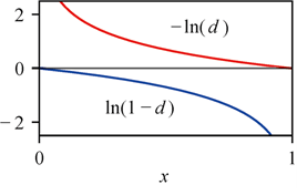
Gradient comparison of the two loss functions: why use -log(d) instead of log(1-d)
In short: the horizontal axis is the discriminator’s output (0 = fake, 1 = real). When the generator is poor (), the gradient of is nearly zero (“cannot learn”), whereas the gradient of is large (“learns fast”).
Mode Collapse
Imagine this: You ask someone to draw all kinds of animals, but they find that drawing cats is especially easy to fool the appraiser, so no matter how much you push them, they only ever draw cats. This is mode collapse—the generator “slacks off” and only produces a few kinds of outputs.
Mode collapse is a common and serious problem in GAN training.
- Definition: During training, the generator’s weights may adapt to a state where all latent variable samples are mapped onto a very small, valid subset of outputs in the data distribution. In the extreme case, the generator may only produce one or a few fixed outputs .
- Example: A GAN trained on handwritten digits might learn to only generate the digit “3” while completely ignoring the other digits.
- Consequences: Although the discriminator cannot tell these “3”s apart from real “3”s, it cannot detect that the generator fails to produce the full range of digits. At this point, the discriminator’s output on these “3” samples stabilizes around 0.5 (meaning it is completely unable to distinguish), causing training to stop and the generator to be unable to improve further.
- Cause: This usually occurs when the discriminator becomes too powerful, or when the generator finds a shortcut that can stably “fool” the discriminator.
The Zero-Gradient Problem
In plain words: At the very beginning of training, the forger is so bad that the appraiser can tell real from fake at a glance. The feedback the forger gets is “you’re too fake,” but there is no specific direction for improvement—like a student who scores zero on an exam but the teacher only says “wrong” without telling them where they went wrong. This is the vanishing gradient problem.
A fundamental difficulty in training a GAN is that when the generated distribution and the real data distribution differ greatly, the discriminator is easy to train, and its gradient signal becomes extremely weak.
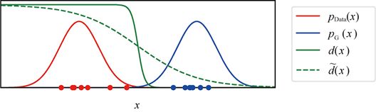
When the two distributions are far apart, the discriminator is nearly zero in the region of generated samples, causing the gradient to vanish
The figure above shows the problem:
- is the distribution of the real data (e.g., a Gaussian distribution).
- is the generator’s initial distribution (e.g., another Gaussian far away).
- The discriminator function outputs close to 1 near the real data and close to 0 near the generated samples.
Mathematical analysis of vanishing gradients
Because the two distributions are far apart, the optimal will be very close to 0 in the region of generated samples. Consider the second term in the generator’s original loss function: .
- When , .
- More importantly, has a very small gradient in this region (it is nearly flat), causing the gradient of the generator parameters to also be very small.
- As a result, the generator’s learning process is very slow, or even stalls.
Improvements
To address training difficulties, researchers have proposed various improvement methods.
Least-Squares GAN (LSGAN)
In short: Change the discriminator’s criterion from a “real/fake probability” to a “score,” using the score gap to provide gradients to the generator.
- Use a smoother discriminator function so that it has stronger gradients in the region of generated samples, thereby providing more effective learning signals to the generator.
- Least-Squares GAN (Least-Squares GAN, LSGAN):
- Modify the discriminator so that it outputs a real-valued number rather than a probability .
- Replace the cross-entropy loss with a least-squares loss: where and are target values (e.g., ). This loss function produces larger gradients when far from the target value, helping to alleviate the vanishing gradient problem.
Input Noise
- Add Gaussian noise to both the real data and the synthetic samples.
- Effect: This makes the data points no longer concentrate at discrete locations but spread out over a small region. This forces the discriminator to learn a smoother decision boundary, thereby avoiding steep, zero-gradient cliffs in the region of generated samples.
Wasserstein GAN (WGAN)
Imagine this: Suppose is a pile of earth and is the target terrain. The Wasserstein distance is the minimum “work” (volume of earth × distance) needed to move that pile of earth to the target location. This distance can tell you “how far apart” even when the two piles of earth do not overlap at all, whereas the original GAN’s loss has already “gone on strike” in this situation (gradient is zero).
- Directly measure the distance (the Wasserstein distance, also known as the Earth Mover’s Distance) between the generated distribution and the real distribution , and let the generator minimize this distance.
- Implementation (WGAN):
- Use a discriminator that outputs real values (now called the Critic).
- Use Gradient Penalty to constrain the norm of the discriminator function’s gradient (to keep it close to 1), which guarantees that the discriminator is 1-Lipschitz continuous (i.e., its rate of change is bounded above), so that it can approximate the Wasserstein distance.
Loss function of WGAN-GP
The loss function of the gradient-penalty Wasserstein GAN (WGAN-GP) is: where is a point sampled randomly between the real and generated data, and is the weight of the penalty term. The first two terms estimate the Wasserstein distance, and the third term ensures the discriminator satisfies the Lipschitz constraint.
Image Generative Adversarial Networks
Deep Convolutional GAN (DCGAN)
Remember the CNN from Part 5? DCGAN is simply applying the convolutional structure of a CNN to a GAN.
DCGAN is an important milestone in the history of GANs, proving that GANs can generate high-quality images.
- Architecture: Uses a standard convolutional neural network (CNN) as the generator and discriminator.
- Generator: Starts from a low-dimensional latent vector and gradually generates a high-resolution image through a series of Transposed Convolution (a kind of “reverse convolution” used to upscale a small image) layers.
- Discriminator: A standard CNN classifier that takes an image as input and outputs a scalar probability.
- Training stability: Through techniques such as batch normalization and appropriate nonlinear activation functions (such as ReLU and Leaky ReLU), DCGAN trains more stably than early GANs.
CycleGAN
Imagine this: You have many photos of horses and photos of zebras, but no paired photos of “the same horse turned into a zebra.” CycleGAN can still learn to turn horses into zebras! Its trick is “cycle consistency”—turn a horse into a zebra and then back into a horse, and you should get the original horse.
CycleGAN is a model for Unpaired Image-to-Image Translation.
- Problem: We have two image domains (e.g., photos of horses) and (e.g., photos of zebras), but no paired samples (i.e., no paired images of “the same horse turned into a zebra”).
- Goal: Learn a mapping that can transform an image from domain into domain , and vice versa .
- Adversarial loss:
- Introduce two discriminators and .
- tries to distinguish real -domain images from images generated by .
- tries to distinguish real -domain images from images generated by .
- Cycle Consistency Loss:
- To ensure the translation is reasonable, a cycle consistency constraint is introduced. An image from domain transformed into domain and then back into domain should yield an image very similar to the original image (“after a round trip, it is still the same”).
Mathematical form of the cycle consistency loss and the total loss
Cycle consistency loss: where is the L1 norm (sum of absolute values), which preserves image detail better than the L2 norm.
Total loss:
where is the weight of the cycle loss.
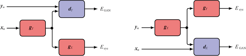
Information flow through CycleGAN. The total error of data points xn and yn is the sum of the errors of their 4 components
Semantic Structure of the Latent Space
A surprising finding is that the latent space of a trained GAN spontaneously organizes itself into a semantically meaningful structure.
- Smooth interpolation: If you walk along a smooth path in the latent space from to , the generated images will smoothly transition from one scene to another, and the intermediate images all look reasonable.
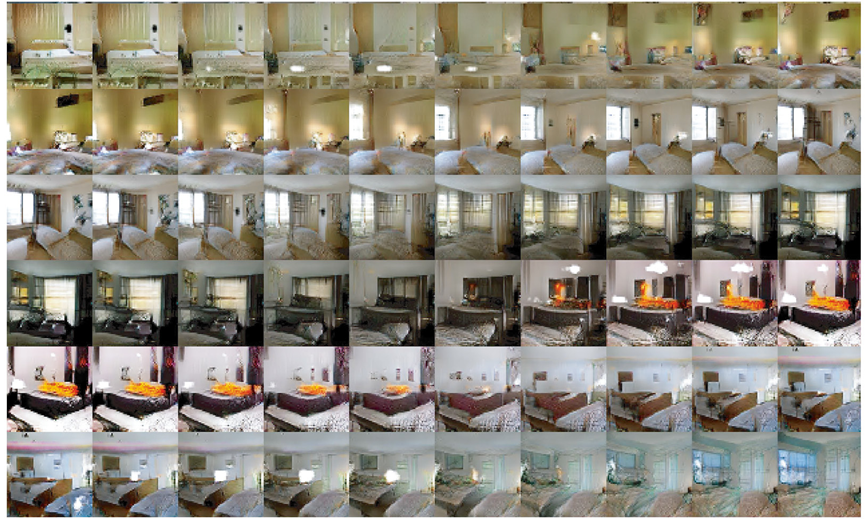
Obtained by smoothly moving between randomly generated positions inside the latent space
- Disentangled Representation: One can find specific directions in the latent space that correspond to semantically meaningful transformations—such as changing the degree of smiling, changing hair color, changing age, etc.
- Example (human faces):
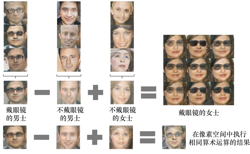
- Example (human faces):
Exercise 1
Background: The training objective of a GAN is a minimax game: .
Why is a GAN so hard to train? And what is “mode collapse”?
Training a GAN is like two people in an “arms race”: once the discriminator gets strong, the generator’s gradient signal gets worse; once the generator gets strong, the discriminator has to upgrade. The two sides must progress in sync, but in practice it is easy for one side to crush the other, causing training to collapse.
Mode collapse: the generator learns to “slack off”—it only generates a few kinds of samples that can fool the discriminator, such as only outputting “1” and “7” when generating digits, and ignoring all the other digits. It finds a shortcut but does not truly learn the data distribution.
What problem does WGAN solve by using the Wasserstein distance instead of the JS divergence?
The JS divergence has a fatal bug: as long as two distributions do not overlap (which is almost always the case in high-dimensional spaces), the JS divergence is a constant , with zero gradient, and the generator simply cannot learn.
The Wasserstein distance (earth-mover distance) is different—even if the two distributions do not overlap, it can still tell you “how far the earth must be moved,” and the gradient is always meaningful. Training is more stable, and the loss value can truly reflect generation quality.
Chapter 17 Summary
One-sentence version: A forger (generator) and an authenticator (discriminator) keep playing against each other, until eventually the forger can produce works that pass as genuine.
Knowledge map:
- Core idea: The minimax game between generator and discriminator
- Key problems: Mode collapse, vanishing gradients, training instability
- Improvement path: LSGAN (smooth loss) -> WGAN (Wasserstein distance) -> CycleGAN (unpaired translation)
- Interesting property: The latent space has a semantic structure and allows “arithmetic” (e.g., smiling man - man + woman = smiling woman)
Chapter 18 Normalizing Flows
Imagine this: You have a ball of clay with a very simple shape (say, a sphere). A normalizing flow is a series of reversible “pinch” and “stretch” operations that turn this simple ball of clay into any complex shape you want (say, a horse). The key point is that every step is reversible—you can also pinch the horse back into a ball. This is the core idea of normalizing flows: through a series of reversible transformations, “morph” a simple distribution into a complex distribution.
Remember the change-of-variables formula from Part 7? The mathematical foundation of normalizing flows is exactly the change of variables in probability theory: when you apply a reversible transformation to a random variable, the probability density of the new variable can be computed via the Jacobian determinant (which measures how much the transformation scales volume).
The goal of this chapter is to design a class of invertible functions that can serve as transformation layers in a generative model. These models are called Normalizing Flows. The key requirements are:
- Invertibility: Given the output , the input must be computable uniquely.
- Easily computable Jacobian determinant: To compute the density transformation, we need to know the determinant of the transformation’s Jacobian matrix . This computation must be efficient.
Consider a simple linear transformation:
Its inverse transformation is:
Although it is invertible and the Jacobian determinant is easy to compute (), it has a fundamental problem: linear transformations are closed under composition. This means that no matter how many linear transformation layers you stack, the overall effect is still a linear transformation. Just as no matter how you stack stretching and rotation, the shape of the clay is essentially still simple. Therefore, even with multiple layers, you can only generate Gaussian distributions and cannot capture complex, non-Gaussian data distributions.
Coupling Flow
Imagine this: You split the ball of clay into left and right halves. The left half stays put first, and the right half is “pinched” according to the shape of the left half—if the left is round, the right is stretched; if the left is flat, the right is compressed. Then you swap roles: the right stays put, and the left is “pinched” according to the right. After alternating a few times, the ball of clay becomes a complex shape!
To solve the insufficient expressiveness of linear transformations, we introduce the Coupling Flow, using Real NVP (Real-valued Non-Volume Preserving) as an example.
- Core idea: Split the latent variable vector into two parts , with dimensions and . Apply different transformations to the two parts.
- Transformation rules:
- The first part is copied directly to the output (the “unchanged half”):
- The second part undergoes an affine transformation (scaling + translation), but the transformation’s parameters (translation and scaling ) are nonlinear functions of : where denotes the Hadamard Product (element-wise multiplication). and are scaling and translation vectors computed by a neural network. The exponential function ensures the scaling factor is positive, guaranteeing the transformation is invertible.
Mathematical derivation of invertibility and the Jacobian determinant
Proof of invertibility: Given the output , the input can be recovered uniquely: 1. (direct copy). 2. Compute and . 3. .
Jacobian matrix and determinant: The Jacobian matrix can be written in block form as a lower triangular matrix:
Since is a lower triangular matrix, its determinant equals the product of the elements on the main diagonal: The key point is that the determinant does not depend on the complex term, but only on the scaling factor . This makes the computation very efficient.
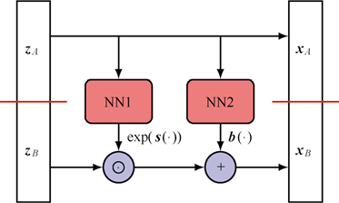
Single-layer structure of the Real NVP normalizing flow model
Stacking Multiple Layers
A single layer of Real NVP has an obvious limitation: is left unchanged in the transformation (“half the clay is not pinched”). This limits the model’s expressiveness.
- Solution: Stack multiple coupling layers and swap the roles of and at each layer.
- First layer: unchanged, transformed.
- Second layer: unchanged, transformed.
- Effect: Through this alternation, each part of the variables will be transformed at different layers. After stacking enough layers, the model can learn very complex, nonlinear invertible transformations.
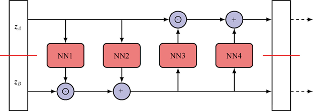
Stacked coupling flows: through alternately swapping roles, all variables get transformed
Autoregressive Flow
Imagine this: When painting, you first paint the sky (), then decide what color to paint the grass () based on the color of the sky, then decide what color to paint the house () based on the sky and the grass… The value of each pixel depends on the pixels already painted before it. This is the idea of “autoregression.”
The inspiration for autoregressive flows comes from a basic fact in probability theory: any multidimensional joint distribution can be decomposed into a product of a series of conditional distributions.
- Joint distribution decomposition: For a -dimensional vector , its joint probability can be written as: where denotes the subvector from to . This requires us to impose a fixed ordering on the variables.
Masked Autoregressive Flow (MAF)
The Masked Autoregressive Flow (MAF) directly uses the above decomposition to construct an invertible generative model.
- Transformation rule: MAF defines a transformation from the latent variable to the data :
- is the -th component of the latent variable .
- is a conditioner, usually a neural network, that predicts the transformation’s parameters based on the preceding .
- is a coupling function that combines and the conditioner’s output to produce . This function must be invertible with respect to .
- Key point: depends only on and the preceding , not on the following .
- Masking: To implement this “depends only on preceding variables” constraint in a neural network, we can use a mask. By setting specific values to zero in the neural network’s weight matrix, we force the network to ignore the information of when computing .
MAF vs IAF: A Trade-off in Efficiency
In plain words: MAF and IAF are like two sides of the same coin. MAF is “fast at computing probability, slow at generating,” while IAF is “fast at generating, slow at computing probability.” Which one you choose depends on your task.
Masked Autoregressive Flow (MAF)—efficient likelihood computation, inefficient sampling:
- Given a data point , we can efficiently compute its log-likelihood —because all can be computed in parallel ( is known).
- But sampling from MAF is very slow, because the generation process must follow the strict order , with each step having to wait for the previous step to complete, giving a time complexity of .
Inverse Autoregressive Flow (IAF)—efficient sampling, inefficient likelihood computation:
- The transformation rule becomes —the conditioner depends on the latent variables rather than the data variables .
- Since can be sampled all at once, all can be computed in parallel, making sampling very fast.
- But computing the likelihood (the inverse transformation) requires serial solving, because computing requires knowing first.
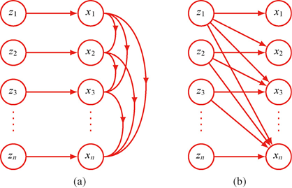
Two autoregressive normalizing flow structures, (a) masked autoregressive flow allows efficient evaluation of the likelihood function, (b) inverse autoregressive flow allows efficient sampling
Basis for choosing:
- If you need to quickly evaluate the probability of a data point (e.g., density estimation, anomaly detection), choose MAF.
- If you need to quickly generate large numbers of samples (e.g., image generation), choose IAF.
Relationship to coupling flows: Autoregressive flows and coupling flows are closely related. A coupling flow can be seen as a special case of an autoregressive flow—it splits the variables into two groups ( and ) rather than groups. This sacrifices some expressiveness, but greatly improves computational efficiency (since the transformations within each group can be parallelized).
Continuous Flows
Neural ODE
Imagine this: A normal neural network is like walking up stairs—one step at a time, jumping discretely. A Neural ODE, on the other hand, is like taking an elevator—rising smoothly and continuously.
Traditional neural networks and normalizing flow models are all composed of discrete layers. The Neural ODE (Neural Ordinary Differential Equation) offers a brand-new perspective: viewing the network as a continuous dynamical system.
- Core idea: Instead of defining a series of discrete transformations , we define a vector field (Vector Field, describing the direction and speed of motion at each point) over a continuous time , where is the state vector at time .
- Differential equation: The evolution of the state is described by an ordinary differential equation (ODE): where is a function implemented by a deep neural network, and are its parameters.
- Initial and final states: Given the initial state , we can integrate this ODE from to to obtain the final state :
- Analogy with traditional networks: This is similar to a residual network (ResNet): When the step size , the discrete residual connection converges to a continuous ODE.
Since is a complex neural network, the ODE usually cannot be solved analytically. We need to use a numerical ODE solver (such as the Runge-Kutta method).
- Process:
- Define the ODE function .
- Provide the initial condition .
- Specify the integration interval .
- Call a black-box ODE solver (e.g.,
scipy.integrate.solve_ivp) to compute .
- Adaptivity of the solver: Advanced solvers (such as
dopri5) are adaptive. They automatically choose the integration step size and time points based on the complexity of the function . This makes the solving process more efficient and more precise.
Backpropagation (Adjoint Method)
The main challenge in training a Neural ODE is computing the gradient of the loss function with respect to the parameters . Chen et al. (2018) proposed an efficient Adjoint Method, whose memory cost is independent of network depth—a huge advantage.
Mathematical details of the adjoint method
- Define the adjoint vector: represents the gradient of the loss with respect to the state at time . At , is the gradient of the loss with respect to the final output , which can usually be computed directly.
- Adjoint equation: itself follows an ODE: This equation can be integrated backward from to .
- Parameter gradient:
Training procedure: 1. Forward pass: Use the ODE solver to integrate from to , obtaining , and compute the loss . There is no need to store the intermediate . 2. Backward pass: Use the reverse ODE solver to integrate the adjoint equation from to , while computing the parameter gradient .
Memory advantage: Since there is no need to store the intermediate states of the forward pass, the memory consumption is constant, whereas the memory consumption of traditional methods is proportional to the network depth.
Neural ODE Flow
A Neural ODE can be used to build a new type of normalizing flow model, called a continuous normalizing flow.
- Transformation: The transformation from input to output is defined by the ODE:
- Density transformation: If we define a simple prior distribution in the input space (such as a standard normal distribution), then through the ODE’s evolution, this distribution propagates to the output space .
- Evolution of the log density: Chen et al. (2018) proved that the log probability density evolves according to another ODE: where is the Jacobian matrix of with respect to , and denotes the trace of a matrix.
- Training: To compute the log-likelihood of the output , we need to solve two ODEs simultaneously:
- , from to .
- , from to . This can be achieved by concatenating the two equations into an augmented system, which is then solved by a single ODE solver.
- Sampling: When sampling from , first sample from , then obtain by solving the ODE.
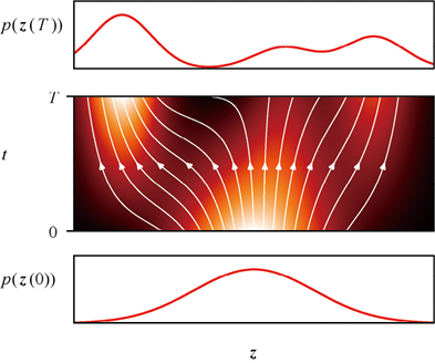
How a simple Gaussian distribution becomes a multi-modal distribution at time t=T through a continuous transformation. When flow lines diverge, density decreases; when flow lines converge, density increases
Exercise 2
What are the respective advantages and disadvantages of normalizing flows and GANs?
Normalizing flows: can compute likelihood exactly (suitable for tasks like anomaly detection that need to know probabilities), and training is stable. But the transformations must be invertible, limiting architecture design, and expressiveness is therefore compromised.
GANs: typically generate higher quality, and the architecture can be designed freely. But likelihood cannot be computed, and training is notoriously difficult.
In short: a normalizing flow is a “well-behaved good student,” while a GAN is a “brilliant but temperamental genius.”
Chapter 18 Summary
One-sentence version: Through a series of invertible transformations, “morph” a simple distribution (such as a Gaussian) into a complex data distribution, just like pinching clay into any shape.
Knowledge map:
- Core idea: Invertible transformation + change-of-variables formula (Jacobian determinant)
- Three architectures: Coupling flow (Real NVP, split into two halves and alternate transformations), autoregressive flow (MAF/IAF, transform dimension by dimension conditionally), continuous flow (Neural ODE, continuous transformation)
- Key trade-off: MAF is “fast at probability, slow at generating,” IAF is “fast at generating, slow at probability”
- Comparison with GAN: Normalizing flows can compute likelihood exactly (GANs cannot), but expressiveness is limited by the invertibility constraint
Chapter 19 Autoencoder
Imagine this: An autoencoder is like “lossy compression.” You compress a high-resolution photo into a small file (encoding), then restore a photo from that small file (decoding). The compression process is “extracting the essence,” and the restoration process is “rebuilding from the essence.” If the restored photo after compression and restoration looks very much like the original, it means the encoder has learned the core features of the data.
Deterministic Autoencoder
An autoencoder is a neural network model aimed at learning effective representations of data. Its core idea is to reconstruct the input data through an “encode-decode” process.
- Network structure: A typical autoencoder consists of two parts:
- Encoder: Maps the input vector to a latent representation (Latent Representation, also called hidden representation) .
- Decoder: Maps the latent representation back to the output vector .
- Training objective: The number of output units equals the number of input units. The training objective is to make the network’s output as close as possible to the original input , thereby learning an identity mapping.
- Latent representation: After training, the hidden layer inside the network (i.e., ) provides a compressed or abstract representation of the input data, which can be used for downstream tasks (such as classification, clustering).
If no constraints are imposed on the network, the simplest solution is for the network to learn an identity function (copying the input directly to the output), which is like “compressing” but the file size does not change—completely useless. To force the network to learn meaningful representations, some form of constraint must be introduced.
- Introducing constraints: Common constraint methods are:
- Dimensionality constraint: Limit the dimension of the latent representation to be smaller than the dimension of the input (i.e., ). This forces the network to perform dimensionality reduction (Dimensionality Reduction), learning the most important features of the data—like compressing 100-dimensional data into 10 dimensions.
- Sparsity Constraint: Even if , regularization (such as L1 regularization) can be used to encourage most elements of to be zero, thereby learning a sparse representation.
- Denoising constraint: By adding noise to the input, train the network to recover the original input from the corrupted input. This forces the network to learn the intrinsic structure and robustness of the data.
Linear Autoencoder
Consider the simplest autoencoder: an input layer, one hidden layer (), and an output layer, with all activation functions being linear.
- Error function: Usually the squared error is used to measure the reconstruction error:
- Equivalence to PCA: When the hidden layer uses a linear activation function, the optimal solution of this autoencoder is equivalent to Principal Component Analysis.
- At the global minimum of the error function, the network projects the input data onto the subspace spanned by the first principal components of the data.
- The weight vectors connected to the hidden units form a basis of the principal subspace (although they are not necessarily orthogonal or normalized).
- Limitation of nonlinear activation functions: Even if a nonlinear activation function (such as sigmoid) is used in the hidden layer, for this two-layer network structure, the optimal solution is still equivalent to linear PCA. This shows that relying solely on a nonlinear activation function cannot break through the limitation of linear dimensionality reduction.
Deep Autoencoder
To achieve true nonlinear dimensionality reduction, deeper network structures need to be introduced.
- Nonlinear mapping: The network can be viewed as two consecutive mappings and :
- : Maps the -dimensional input space to the -dimensional latent space . Due to the presence of nonlinear layers, this mapping can be very complex and is no longer limited to linear transformations.
- : Maps the -dimensional latent space back to the -dimensional output space.
- Geometric interpretation: As shown in the figure below, defines how the latent manifold is embedded into the high-dimensional data space. Since is nonlinear, this embedding can be non-planar, thereby capturing complex nonlinear structures in the data.
- Training challenges: Unlike the linear autoencoder, the error function of a deep autoencoder is no longer a quadratic function of the parameters , so the optimization process is nonlinear. This requires computationally expensive nonlinear optimization techniques, and there is a risk of falling into local optima.
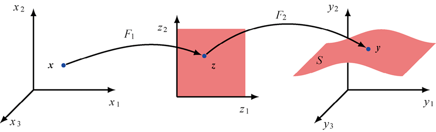
Geometric interpretation
Sparse Autoencoder
Another way to constrain is to encourage the sparsity of the latent representation through regularization.
- L1 regularization: Add an L1 norm term to the error function, penalizing the sum of the absolute values of the latent unit activations: where is the original unregularized error (such as squared error), is the number of hidden units, and is the regularization coefficient.
- Effect: L1 regularization tends to produce sparse solutions, i.e., most values are zero or close to zero. This forces the network to use only a few hidden units to represent the input, thereby learning more interpretable features.
- Gradient computation: Although the regularization term acts on unit activations rather than network parameters, gradients can still be computed efficiently for training through automatic differentiation.
Denoising Autoencoder
Remember the diffusion model later on? The core idea of the denoising autoencoder is very similar to that of the diffusion model—both are “add noise to the data, then learn to remove the noise.” It can be said that the denoising autoencoder is the intellectual predecessor of the diffusion model.
A denoising autoencoder learns robust representations of data by learning to recover the original input from a corrupted input.
- Training process:
- Take an original input vector .
- Apply noise to it (such as randomly zeroing some inputs, or adding Gaussian noise), obtaining a corrupted version .
- Feed as input to the autoencoder, obtaining the output .
- The training objective is to minimize the error between the output and the original, uncorrupted input :
- Learning mechanism: By learning to “denoise,” the network is forced to discover the statistical regularities and intrinsic structure in the data. For example, in image data, it learns that adjacent pixels are highly correlated, so it can use the information of surrounding pixels to repair the corrupted pixels.
- Relationship with score matching: The training of a denoising autoencoder is closely related to Score Matching. The score function is an “arrow” pointing toward regions of high data density. The reconstruction direction learned by the denoising autoencoder also points toward the data manifold, similar to the score vector. This connection will reappear in the diffusion model chapter.
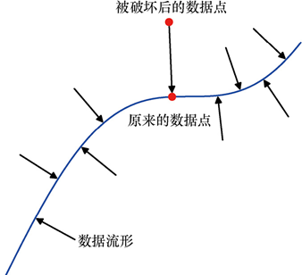
In a denoising autoencoder, data points are assumed to lie on a low-dimensional manifold in the data space, and are corrupted by additive noise. The autoencoder learns to map the corrupted data points back to their original values, so the autoencoder learns a vector pointing toward the manifold for every point in the data space
Masked Autoencoder (MAE)
Remember the Transformer from Part 6? MAE applies the Transformer to images—it splits the image into small patches (patch), just like splitting text into tokens, then randomly masks out most of the patches and lets the model learn to recover them.
The Masked Autoencoder is a special form of the denoising autoencoder, especially suitable for images and Transformer-based architectures.
- Masking operation: The input image is divided into multiple “patches.” During training, a portion of the patches is randomly selected and “masked” or discarded (e.g., 75%). Unlike BERT, instead of replacing them with a fixed “mask token,” these patches are directly omitted.
- Architecture: Usually combined with a vision Transformer.
- Encoder: Receives the unmasked patches as input and computes their representations.
- Decoder: Needs to reconstruct the entire image (including the masked patches). To achieve this, between the encoder and the decoder, the masked patches must be re-inserted using a fixed mask token vector (with positional encoding attached) to restore the original sequence length.
- Training objective: The loss function only computes the reconstruction error on the masked patches (such as mean squared error). The decoder is trained to predict the original pixel values of these missing patches.
- Advantages:
- Computational efficiency: Since the encoder only processes the unmasked patches (e.g., 25%), the computation is greatly reduced.
- Powerful representation learning: By predicting large missing regions of the image, the encoder is forced to learn the global semantics and structural information of the image.
- Downstream tasks: After training, the decoder is discarded. The encoder (possibly with new output layers attached) is used for downstream tasks such as image classification and detection.
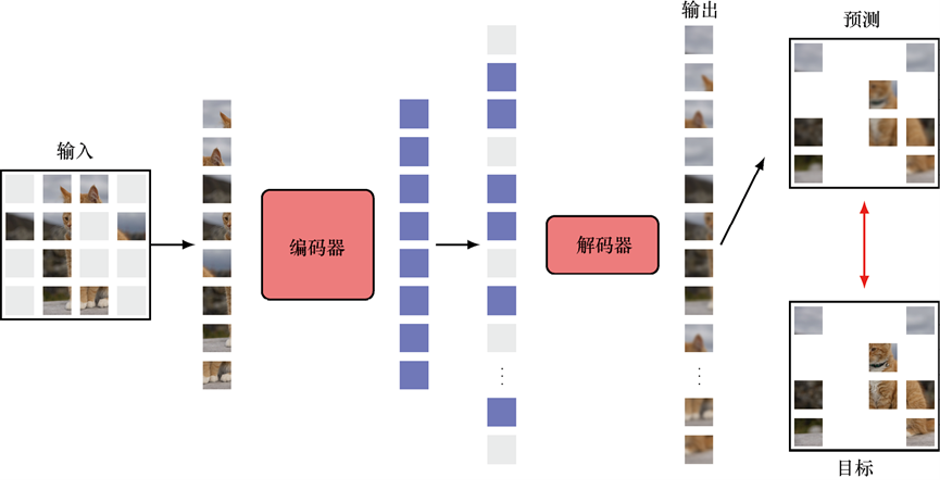
Architecture of the masked autoencoder in the training phase. After training, the decoder is discarded, and the encoder is used to map images to internal representations for use in subsequent tasks
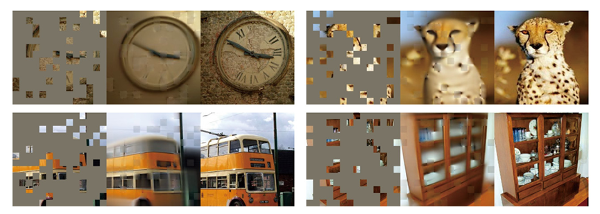
The masked image is on the left (80% of input patches masked), the reconstructed image is in the middle, and the original image is on the right
Variational Autoencoder (VAE)
Imagine this: A normal autoencoder is “lossy compression”—it compresses a picture into a fixed vector. A VAE goes further: instead of compressing it into a fixed vector, it compresses it into a probability distribution (such as a Gaussian distribution with “mean here, and variance this large”). To generate a new picture, you only need to randomly sample a point from this distribution, then decode it.
Remember variational inference and ELBO from Part 7? The mathematical foundation of the VAE is exactly variational inference—using a simple distribution to approximate the complex posterior distribution , and maximizing the ELBO.
The Variational Autoencoder (VAE) is a probabilistic generative model that approximates a complex posterior distribution through variational inference.
- Generative model: A VAE defines a latent variable model—the way to generate data is: first sample from a simple distribution, then generate through the decoder: where is the prior distribution (usually a standard normal distribution ), and is the likelihood function defined by the decoder neural network.
- Difficulty of posterior inference: Directly computing the posterior distribution is difficult, because the marginal likelihood cannot be computed analytically (it requires integrating over all possible ).
To solve the difficulty of posterior inference, the VAE uses the Evidence Lower Bound (ELBO) to approximately maximize the log-likelihood.
- Optimization objective: Maximize the ELBO , which is equivalent to minimizing the KL divergence (a measure of the difference between two distributions) between the approximate posterior and the true posterior .
Amortized Inference
For efficient learning, the VAE uses a neural network (the encoder) to approximate the posterior distribution for all data points.
- Encoder network: Introduce a parameterized encoder network , which maps the input to a distribution (usually a Gaussian) of the latent variable .
- Parameterization: A typical encoder outputs a diagonal Gaussian distribution’s mean and variance :
- Joint optimization: Now, the ELBO depends on both the decoder parameters and the encoder parameters . The objective is to jointly optimize .
Reparameterization Trick
In plain words: The problem is this—a neural network needs to learn through “backpropagation,” but the “sampling” operation is like a wall that gradients cannot pass through. The clever trick of the reparameterization trick is: separate the “random sampling” from the parameter computation. It is like saying “I don’t sample directly from the distribution, but first sample a fixed random number, then compute the sampling result with a formula”—this way the gradient can flow back through the formula.
Direct gradient descent on the ELBO is difficult, because the sampling operation blocks backpropagation.
- Problem: The ELBO contains an expectation term, which needs to be approximated by Monte Carlo methods (Monte Carlo, i.e., stochastic sampling approximation): But is sampled from , and depends on , so the gradient cannot pass through the sampling operation to the encoder.
- Solution: The reparameterization trick separates the randomness from the parameter dependence.
- For a Gaussian distribution, the sampling can be expressed as:
- Now, explicitly depends on and (i.e., ), while is an independent noise source unrelated to the parameters.
- This allows the gradient to backpropagate through and to the encoder network.

Fixing the latent variable z to a specific sampled value prevents the error signal from backpropagating to the encoder network
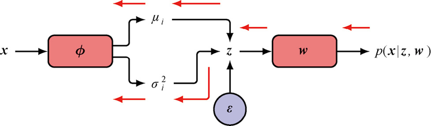
The reparameterization trick allows the error signal to backpropagate to the encoder network by computing from a sample of an independent random variable e instead of sampling z directly
Combining all the above parts, the complete ELBO objective function of the VAE can be written as:
Mathematical form of the VAE's complete ELBO objective function
where (reparameterization), , . Usually , i.e., each data point is sampled only once.
Intuition: The ELBO consists of two parts—the KL divergence term ensures the distribution output by the encoder does not deviate too much from the standard normal distribution (regularization), and the reconstruction term ensures the decoder can restore the original data from the latent variable (fidelity). A balance must be struck between the two.
Exercise 3
What does the VAE’s “reparameterization trick” do? What would happen without it?
The VAE’s encoder outputs a distribution (mean + variance), and when generating the latent variable, we sample from this distribution. The problem is: the sampling operation cannot be differentiated—the gradient cannot flow back to the encoder.
The reparameterization trick is clever: set , where is noise sampled from the standard normal. This way the randomness is transferred to , and the gradient can backpropagate normally through and .
Without this trick, the VAE could not train the encoder with gradient descent, and could only use high-variance methods like REINFORCE, making training very painful.
Can a normal autoencoder generate new data? Why can a VAE?
A normal autoencoder cannot. Its latent space is unconstrained, and the latent variables of data points are scattered all over the place; if you randomly sample a point from the latent space, what you decode is most likely garbage.
The VAE “tidies up” the latent space into something close to a standard normal distribution through the KL divergence—continuous, smooth, and organized. Sampling any point from this latent space and decoding it produces meaningful data. This is why the VAE can serve as a generative model.
Chapter 19 Summary
One-sentence version: An autoencoder learns to “compress-decompress” data; the VAE upgrades it to a probabilistic version—compressing into a distribution rather than a point, so that it can generate new data.
Knowledge map:
- Deterministic autoencoder: Encoder + decoder, learning meaningful representations through constraints
- Linear autoencoder ≈ PCA
- Deep autoencoder: true nonlinear dimensionality reduction
- Sparse autoencoder: L1 regularization encourages sparsity
- Denoising autoencoder: recovering original data from noise (connected in idea to the diffusion model)
- Masked autoencoder: Transformer + large-area occlusion
- Variational Autoencoder (VAE): Encode into a distribution, train with ELBO, reparameterization trick lets gradients propagate
- Comparison with GAN: VAE training is stable but generated images tend to be blurry; GAN training is difficult but generation quality is high
Chapter 20 Diffusion Models
Imagine this: You are calling a friend, and the signal is clear at first (the original image). Then someone gradually adds more and more noise to the phone line (forward noising), until you can no longer hear what the other person is saying (it becomes pure noise). What a diffusion model does is: learn how to step by step restore a clear signal from a pile of noise (reverse denoising).
You may ask: “Anyone can add noise? Removing noise is the hard part, right?” Exactly! The cleverness of the diffusion model lies in: although the forward noising is fixed and does not need to be learned, each step of the reverse denoising is very small, so small that a neural network can easily learn it.
The Diffusion Model is currently a generative model framework that achieves SOTA (State-of-the-Art) results in fields such as image generation. Its core logic can be summarized as “forward noising -> reverse denoising”:
- Forward Process (Forward Process, encoder): Gradually “corrupt” the training data (such as images) through multiple steps of additive Gaussian Noise, eventually turning the data into samples from a standard Gaussian distribution (completely devoid of original data information);
- Reverse Process (Reverse Process, decoder): Train a deep neural network to learn to reverse the above noising process—starting from a standard Gaussian sample, denoise step by step, and finally generate new samples consistent with the training data distribution.
Comparison with GAN and VAE: A diffusion model can be viewed as a kind of “Hierarchical VAE”—the distribution of the forward noising is fixed (no need to learn), and only the generative distribution of the reverse denoising needs to be learned. Compared to GANs, it avoids the instability of adversarial training, and training is simple and easy to parallelize; but generating samples requires multiple passes through the decoder (usually hundreds to thousands of steps), so the computational cost is higher.

Forward noising process: starting from the original image x, after T steps of noising we get z_T close to a Gaussian distribution, and the reverse process is to gradually denoise from z_T back to x
Forward Encoder
In plain words: The forward encoder is the “rule for adding noise.” At each step, you sprinkle a bit of Gaussian noise onto the picture (like sprinkling sand onto a photo). One sprinkle is not too blurry, but after hundreds of sprinkles, the photo becomes a field of random sand grains—you can no longer tell what it originally was.
The forward encoder defines “how to gradually add noise to the data.” The whole process is a Markov Chain (i.e., each step depends only on the result of the previous step, not on earlier history), as follows:
For an original image in the training set, the first noising step mixes with independent Gaussian noise to obtain the first noisy image :
where:
- : standard Gaussian noise (mean 0, identity covariance matrix);
- : Noise Variance, controlling the strength of the first noising step. The smaller is, the weaker the noising, and the smaller the change to the image;
- The role of the coefficients and : ensures that the mean of is closer to 0 than , and the covariance is closer to the identity matrix than (paving the way for the subsequent multi-step noising to eventually converge to a standard Gaussian).
From the perspective of probability distribution, the conditional distribution of given is a Gaussian distribution:
Repeating the single-step noising times gives the noisy sequence , and the noising rule at each step is consistent with the first step:
where , and each is an independent new noise.
The corresponding conditional distribution is:
Parameter setting: needs to be set manually (called the noise schedule), usually following (weak noising early, strong noising later), ensuring that when is large enough, approaches a standard Gaussian.
The forward noising process can be represented as a probabilistic graphical model:
- Shaded node : observed variable (original image, known);
- Blank nodes : latent variables (noisy images, unknown);
- Forward distribution : defines the noising direction (encoder, known);
- Target-to-learn reverse distribution : defines the denoising direction (decoder, are the network parameters, to be learned);
- Conditional distribution : given the original image , the distribution of inferring from —this is the key to deriving the training objective.
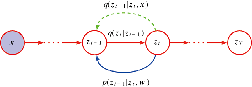
Probabilistic graphical model of the diffusion model: x is the known original image, and z_1 to z_T are the gradually noised latent variables
Diffusion Kernel (Marginal Distribution of )
In plain words: The diffusion kernel tells you some good news—during training you don’t need to actually add noise step by step all the way to step ; you can get there in one shot by directly generating the step- noisy image from the original image . This greatly speeds up training!
In the forward process, if you want to directly obtain (without computing the intermediate ), you can do so through the “marginal distribution.” The conditional distribution of given (called the Diffusion Kernel) is a Gaussian distribution:
where is the cumulative product of (the proportion of signal retained):
Derivation idea of the diffusion kernel
- The joint distribution of the forward process is (Markov chain property);
- Integrating out , and using the property that “the sum of independent Gaussian variables is still Gaussian,” we can derive that the mean of is , and the variance is .
Training significance: The diffusion kernel lets you jump directly to any step during training, without running the full forward chain, greatly improving training efficiency.
The diffusion kernel can also be rewritten in noising form (which is very useful when deriving the loss function later):
Note: here is the “accumulated noise” (the total noise from to ), rather than the single-step noising .
Limit case: When the number of noising steps , , and the diffusion kernel becomes — is completely standard Gaussian noise, with nothing to do with the original image . This is what we want: the forward process eventually “erases” all the original information.
Conditional Distribution (the “Ground Truth” for the Reverse Process)
In plain words: We want to train a neural network to “denoise,” but it needs a “ground truth” to learn from. The conditional distribution is exactly this ground truth—it tells you “if you know what the original image is, then how should you recover from .”
Our goal is to learn the reverse denoising (from to ), but directly inverting gives , which requires knowing (the data distribution) that we don’t know, so it cannot be computed. Therefore, we consider the “reverse conditional distribution given ” —the good news is that this distribution is a simple Gaussian!
Derivation process of the conditional distribution
Apply Bayes’ Theorem:
Simplify using the Markov property: the forward process is a Markov chain, so , and both and are diffusion kernels.
Since both numerator and denominator are Gaussian distributions, is also Gaussian:
where:
- Mean :
- Variance (depends only on and , unrelated to ):
Significance of this distribution: It provides a “target distribution” for training the neural network—during training, make the reverse distribution predicted by the network as close as possible to this “ground truth” .
Reverse Decoder
In plain words: The reverse decoder is that “denoiser”—a neural network that takes the noisy image and the current step number as input and outputs the denoised mean. It is the core part of the diffusion model that needs to be trained.
The core of the reverse decoder is “learning a deep neural network that approximates the reverse denoising process corresponding to ,” and through this network generate (a clear data sample) from (pure noise).
Directly computing is infeasible (it requires integrating over all possible ), so we model the reverse distribution with a neural network, in the form of a Gaussian distribution:
where:
- : the mean output by the deep neural network ( are the network parameters, and is input to adapt to different noise intensities);
- Variance set to : referencing the variance of the forward noising, and when is small, the reverse distribution approximates a Gaussian, with variance close to .
On network architecture: The output dimension of the neural network must match the input ()—in image data, this is the image size. The commonly used architecture is U-Net—an encoder-decoder structure with skip connections, suitable for capturing both local and global features of images. In recent years, Transformer architectures have also been used.
Choice of : Why “Small Steps, Slow Walk”?
Imagine this: If you add a lot of noise at once ( large), it’s like blurring the photo all at once—when denoising, it’s hard to guess what the original was. But if you add only a little noise each time ( small), the change at each step is small, and the neural network can easily learn to “remove this step’s blur.”
It is recommended to set (weak noising at each step), for the following reasons:
- In the forward noising, a small means and differ little, so the “correction magnitude” in reverse denoising is small, making it easier for the network to learn;
- The reverse distribution will approximate a Gaussian:
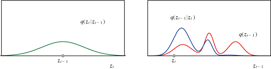
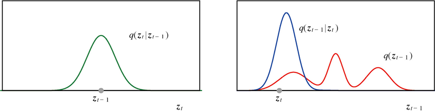
- Top figure: when is large, is a multi-modal distribution (complex, hard for the network to model);
- Bottom figure: when is small, is close to Gaussian (simple, easy to model).
The cost: a large number of steps (usually hundreds to thousands) is needed for to approach a standard Gaussian, causing high computational cost when generating samples. This is the fundamental reason why diffusion models are “fast to train, slow to generate.”
Joint Distribution of the Reverse Process
The entire reverse denoising process is a Markov chain, with joint distribution:
where:
- (consistent with the forward process’s );
- : the distribution of finally generating (no noise) from (weak noise), in a form similar to (Gaussian distribution).
Training Objective: Evidence Lower Bound (ELBO)
Remember the VAE’s ELBO? The diffusion model uses exactly the same idea—directly maximizing the log-likelihood is too hard (it requires integrating over all possible noise paths), so we maximize a lower bound of it, the ELBO.
The ideal training objective of a generative model is to maximize the log-likelihood of the data, but this likelihood requires integrating over all latent variables , involving complex neural networks, and cannot be computed directly. Therefore, borrowing the idea of the VAE—maximize the lower bound (ELBO) of the likelihood.
For any latent variable distribution , we have:
where is the ELBO, and . Therefore , and maximizing indirectly maximizes the likelihood.
Choose (the fixed distribution of the forward process), substitute into the ELBO and simplify, and finally decompose it into a “reconstruction term” and a “consistency term”:
Complete derivation of the ELBO
- Reconstruction term: Rewards the network’s ability to reconstruct the original data (similar to the VAE’s reconstruction loss).
- Consistency term: Ensures the reverse distribution is as consistent as possible with the target distribution (by minimizing the KL divergence).
Since the KL divergence between two Gaussian distributions has an analytical solution, the consistency term can be simplified to a squared loss: where is the mean of the “ground truth,” and is the mean output by the network.
In short: The ELBO consists of two parts—the reconstruction term requires “recovering the original image from very little noise,” and the consistency term requires “accurate denoising at every step.” The consistency term is the core of diffusion model training.
Key Improvement: Predict Noise Instead of the Denoised Image
You may ask: Why make the network predict noise instead of directly predicting the denoised image? In plain words: noise is much simpler than an image. Imagine a painting covered by sand—it’s hard to guess the full picture, but it’s relatively easy to guess “how much sand is on it.” And once you know the distribution of the sand, removing the sand is simple.
In practice, changing the network’s target from “predict the denoised image ” to “predict the accumulated noise ” can significantly improve generation quality.
Why predicting noise is equivalent to predicting the denoised image (mathematical derivation)
From the diffusion kernel formula , solve for :
Rewrite the mean of as a function of :
If we define a network that predicts the accumulated noise , then the relationship between the network output and is:
After integration, the final training objective is simplified to (omitting the weight factor, which is found empirically to improve performance):
Intuition of the loss function: For each training sample and a random time step , sample noise to generate , let the network predict “what noise was added,” and the loss is the squared difference between the “predicted noise” and the “true noise.” The training objective is very simple and clear!
Training and Generation Algorithms
In plain words: Training does one thing repeatedly—randomly pick an image, randomly add some noise, let the network guess “what noise was added,” then adjust the network to make it guess more accurately. Generation is the reverse—start from pure noise, let the network step by step guess “what noise was added this step,” then remove that noise.
Training process:
- Preprocessing: Set the noise schedule , and compute for each ;
- Iterative training:
- Sample a data sample from the training set;
- Randomly sample a time step (to avoid computing for all , improving efficiency);
- Sample standard Gaussian noise ;
- Compute the noisy sample ;
- Compute the loss , and update the network parameters via stochastic gradient descent;
- Termination: Until the loss converges.
Generation process (sampling):
- Sample pure noise from ;
- From down to , denoise step by step:
- The network takes and as input and outputs the predicted noise ;
- Compute the denoised mean , then add a little noise to generate ;
- Final step (): add no noise, and directly output the generated sample .
Problem of generation speed: The main drawback of diffusion models is that generation requires hundreds to thousands of denoising steps, with high computational cost. Improvement directions include:
- Latent Diffusion Model (LDM): First use an autoencoder to compress high-resolution images into a low-dimensional latent space, perform diffusion in the latent space (low dimension, fast computation), and finally decode back to high-resolution images. Stable Diffusion is based on this idea.
- Faster samplers: Methods like DDIM can generate images of similar quality in fewer steps.
Score Matching
Imagine this: You are on a mountain (the “terrain” of the probability density), and the score function draws an arrow under your feet pointing in the “uphill” direction (the direction of increasing probability density). If you know the arrow direction at every point, you can walk along the arrows to the mountaintop (where the probability is highest), which is where data is most likely to appear.
Score Matching is another class of generative model framework, closely related to diffusion models, whose core is “learning the score function” of the data distribution, and then generating samples through Langevin dynamics.
The score function is the gradient of the log probability density with respect to the data:
where:
- denotes the gradient with respect to the data vector (not with respect to the network parameters);
- If is an image, is also an image of the same size (each pixel corresponds to a gradient value).
Significance of the score function: Learning the score function is equivalent to learning the data distribution (up to a normalization constant), and the score function does not need to know the normalization constant—a huge advantage, since the normalization constant is usually incalculable.
Score Loss Function
The objective is to learn a neural network model that is close to the true score function , with the loss function:
Problem: The true score function is unknown—the training data is only a finite number of samples, so cannot be computed directly. The solution is Denoising Score Matching.
Denoising Score Matching
In plain words: The core idea of denoising score matching is the same as the diffusion model—add noise to the data, then learn the “direction of the noise” (i.e., the score function). After adding noise, the score function becomes easy to compute.
Derivation process of denoising score matching
Smooth the data with a Gaussian kernel to obtain the approximate distribution :
where .
Change the loss function to “score matching of the smoothed distribution”:
After simplification, for the Gaussian kernel , its score function is:
Connection with diffusion models: If we combine the noise level of the diffusion model (), then the score function is:
At this point, the score loss is essentially equivalent to the diffusion model’s loss: the score function corresponds to the diffusion model’s noise prediction network (differing only by a constant scaling factor). Therefore, “denoising score matching” and “diffusion model” reach the same goal by different paths!
Langevin Dynamics Sampling
Imagine this: You are on a foggy mountain, can’t see the road, but can feel the slope under your feet (the score function). Langevin dynamics is—at each step you walk a small step in the “uphill” direction, plus a little random “wind” disturbance. After many steps, you will reach the mountaintop (where the probability density is highest).
After training the score model, samples are generated through Langevin Dynamics—using the score function to guide the sampling direction (toward increasing probability density), with the steps:
- Initialize the sample (starting from a standard Gaussian);
- Iteratively update ( to ): where is the step size (a small value, for stability). Each step contains two parts: the “deterministic guidance” of the score function and the “random disturbance” of the noise.
- After iteration terminates, is the generated sample.
Trade-off of a single noise level: If is too small, the score function is undefined outside the data manifold and sampling is unstable; if is too large, over-smoothing distorts the original data distribution.
Solution: Annealed Langevin Dynamics—use a decreasing sequence of noise variances :
- Large : initial sampling starts from the smoothed distribution, avoiding manifold problems;
- Gradually decrease : gradually approach the original data distribution;
- This is completely consistent with the step-by-step denoising logic of the diffusion model!
Stochastic Differential Equation (SDE) Perspective
In plain words: The discrete steps described earlier (adding a little noise at each step) can be generalized mathematically into a continuous process—like turning “climbing stairs one step at a time” into “taking an elevator.” The SDE is the mathematical language that describes this continuous process. The good news is that, with SDEs, we can use more efficient numerical methods to accelerate generation.
When the number of steps of the diffusion model and the noise variance per step , the discrete forward/reverse process can be expressed as a Stochastic Differential Equation (SDE):
Core formulas of the SDE
Forward SDE (noising process):
Reverse SDE (denoising process):
where is the score function, guiding the denoising direction.
Corresponding ODE (deterministic process):
The ODE can use an efficient adaptive step-size solver, greatly reducing the number of function calls and improving generation efficiency.
Key significance: The SDE framework unifies diffusion models, score matching, and Langevin dynamics under one mathematical system—they are different faces of the same coin.
Guided Diffusion
In plain words: The diffusion models described above can only “randomly generate” images—what is generated is entirely up to luck. But in practical applications, we want to “specify” what to generate, such as “generate a cat” or “generate an image based on a text description.” Guided diffusion adds a “navigation” to the diffusion model, steering it to generate in the direction we want.
The diffusion models above are all unconditional generation (Unconditional Generation), but practical applications often require conditional generation (Conditional Generation, such as generating images based on class labels or text descriptions). Guided diffusion controls the generation process by “introducing a guidance signal,” mainly in two ways.
Classifier Guidance
Using a pretrained classifier ( is the condition, such as the class label “cat”), Bayes’ theorem is used to correct the “unconditional score function” into a “conditional score function,” guiding the denoising process toward the target condition.
In short: conditional score = unconditional score + gradient of the classifier (multiplied by a weight):
- : no guidance, degenerates to unconditional generation;
- : strictly follows the conditional distribution ;
- : enhances the guidance strength (generated samples better match , but diversity decreases—“more obedient but more monotonous”).
Mathematical derivation of classifier guidance
By Bayes’ theorem:
Take the gradient with respect to (, since is independent of ):
Disadvantage: Requires additionally training a classifier that can handle noisy images (a standard classifier is only trained on clean data), and the classifier may only focus on local features, affecting overall generation quality.
Classifier-Free Guidance
In plain words: The idea of classifier-free guidance is more clever—no extra classifier is needed; instead, during training we “occasionally deliberately forget the condition.” This way the model learns both “conditional generation” and “unconditional generation” at the same time, and during generation we control the “degree of obedience” by adjusting the ratio between the two.
Without a pretrained classifier, directly train a “condition-uncondition unified model”: during training, randomly blank out the condition of some samples (e.g., , with probability 10%-20%), so that the model learns both (conditional) and (unconditional).
The score function during generation is:
- : a mixture of conditional and unconditional scores;
- : weakens the influence of the unconditional score, forcing generated samples to better match .
Advantages:
- No extra classifier to train, simplifying the pipeline;
- The model focuses on overall features (rather than the classifier’s local features), so generation quality is higher.
This method is currently the most mainstream conditional generation approach; models like Stable Diffusion and DALL-E all use classifier-free guidance.
Application Scenarios
- Text-guided image generation (text-to-image): Change the condition to a text description (prompt), combined with a large language model (such as a Transformer):
- The text is encoded into a vector by the language model and used as an additional input to the diffusion model;
- A cross-attention layer (Cross-Attention) is added to the diffusion model, letting the network attend to the correspondence between text tokens and image features.
Remember the Transformer from Part 6? Cross-attention is exactly the core mechanism of the Transformer—here it is used to let the image “understand” the text description.
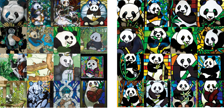
Text-to-image comparison: left $ \lambda=0 $ no guidance, right $ \lambda=3 $ strong guidance
- Image super-resolution: Input a low-resolution image, with the condition being the low-resolution image; the diffusion model starts from high-resolution Gaussian noise and gradually denoises to generate a high-resolution image matching the low resolution.
- Latent Diffusion Model: Solves the computational cost problem of high-resolution image generation:
- Step 1: Train an Autoencoder to compress high-resolution images into a low-dimensional latent space;
- Step 2: Fix the autoencoder and train the diffusion model in the latent space (low dimension, fast computation);
- Step 3: The latent vector generated by the diffusion model is decoded by the autoencoder’s decoder, recovering a high-resolution image.
- Stable Diffusion is based on this architecture!
- Other applications:
- Image inpainting: The condition is “mask of the missing part + the known part of the image,” generating the missing region;
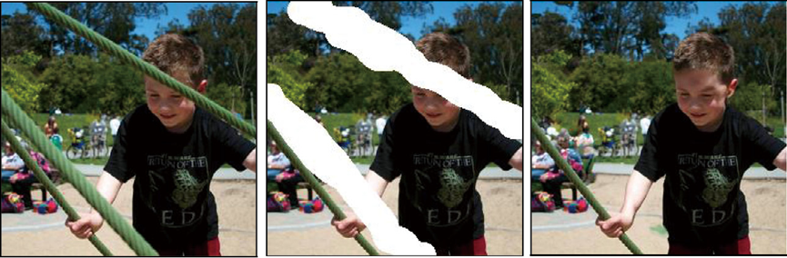
Left is the original image, middle is the masked image, right is the inpainting result
- Image colorization, deblurring, video generation, etc.: all guide the diffusion model to generate the target result by using task-related information as the condition .
Exercise 4
The diffusion model has the network predict noise instead of directly predicting the denoised image. Why is this better?
Imagine a painting covered by sand: it’s hard to guess the full picture, but it’s much easier to guess “how much sand is on it.” Noise is the “sand”—it is simpler than the image, and easier for the network to learn. And once you know the noise, denoising is just subtraction: .
What are the “forward process” and “reverse process” doing, respectively? Why does the forward process not need to be learned?
The forward process is “wrecking”—gradually adding noise to the image until it becomes pure noise. This process is fixed; how much noise to add at each step is predetermined, so it doesn’t need to be learned.
The reverse process is “repairing”—gradually removing noise from pure noise to recover the image. This needs to be learned, because the network has to understand “what is noise” and “what is image structure.”
To use an analogy: sprinkling sand onto a painting (forward) requires no skill, but precisely sweeping the sand off (reverse) requires craftsmanship.
Chapter 20 Summary
One-sentence version: First add noise step by step to turn the image into pure noise, then train a neural network to learn to remove the noise step by step. Like an interfered phone signal—once you know how the noise was added, you can learn how to remove it.
Knowledge map:
- Core idea: Forward noising (fixed) + reverse denoising (needs to be learned)
- Training objective: Have the neural network predict the noise added at each step (rather than directly predicting the denoised image)
- Mathematical framework: ELBO -> score matching -> SDE (the three are essentially equivalent)
- Conditional generation: Classifier guidance (needs an extra classifier) -> classifier-free guidance (mainstream solution)
- Practical application: Stable Diffusion = latent diffusion model + classifier-free guidance + Transformer text encoder
- Advantages: Stable training, high generation quality
- Disadvantages: Slow generation (requires hundreds of denoising steps)