Part 7/8 of the series ← Previous | Next | Glossary

It is recommended to read Parts 1-3 first; Part 4 (optimization methods) will also be helpful. This part covers how to sample from probability distributions, what latent variables are, how PCA performs dimensionality reduction, and how the EM algorithm handles missing data.

Chapter 14 Sampling

Imagine there is a sealed box in front of you, filled with balls of different colors. You want to know the proportion of each color, but you cannot open the box to look — you can only reach in, randomly draw out a ball, record its color, put it back, and repeat many times. This is the core idea of sampling: by drawing samples from a probability distribution that you cannot directly “see”, you learn its properties.

• Definition: Generate samples that follow a probability distribution $p(z)$ (such as generating random numbers from a Gaussian distribution, or generating images from a generative model defined by a deep neural network). Also called Monte Carlo Sampling (a method that uses random experiments to approximate computations).
• Applications: Evaluating expectations, generating synthetic data, training generative models, etc.

Basic Sampling

Expectation

Intuition: Suppose you want to know the average height of the residents in a city. You cannot measure everyone, but you can randomly pick 1000 people, measure them, and compute the average — when the sample is large enough, this average will approach the true value. This is the core idea of the Monte Carlo method: use a large number of random experiments to approximate computations.

• Goal: Compute the expectation of a function $f(z)$ with respect to a distribution $p(z)$ (i.e., a weighted average, where the weights are probabilities): $$\mathbb{E}[f] = \int f(z) p(z) dz \quad (\text{continuous variable}) \quad \text{or} \quad \sum f(z) p(z) \quad (\text{discrete variable})$$
• Monte Carlo Approximation: By drawing $L$ independent samples $z^{(1)}, ..., z^{(L)}$ from $p(z)$, estimate the expectation using the sample mean: $$\overline{f} = \frac{1}{L} \sum_{l=1}^L f(z^{(l)})$$

Sampling from Standard Distributions

Intuition: If you can shake out a random number between 0 and 1, can you “morph” it into a random number from some other distribution? The answer is yes — just like stretching a uniform lump of clay into any shape.

• Inverse Transform Sampling: Use samples from a Uniform Distribution (a distribution where every value has the same probability) to generate samples from other distributions. Let $z \sim U(0,1)$, and apply the transformation $y = g(z)$ so that $y \sim p(y)$, satisfying:

  $$p(y) = p(z) \left| \frac{dz}{dy} \right|$$

  Here $p(z) = 1$ (uniform distribution), so $z = \int_{-\infty}^y p(\hat{y}) d\hat{y} = h(y)$, i.e., $y = h^{-1}(z)$ (where $h(y)$ is the Cumulative Distribution Function (CDF), which represents “the probability of being less than or equal to a certain value”)).

  In short: the inverse of the target distribution’s CDF is the tool that “morphs” a uniform random number into the target distribution.

  • Example: The Exponential Distribution (commonly used to describe waiting times) $p(y) = \lambda e^{-\lambda y}$, whose cumulative distribution is $h(y) = 1 - e^{-\lambda y}$ , so the transformation is $y = -\lambda^{-1} \ln(1 - z)$.
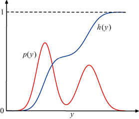
  • The geometric interpretation of generating a non-uniform distribution via the inverse transform method: $h(y)$ is the indefinite integral of the desired target distribution $p(y)$. If we transform the uniformly distributed random variable z using $y = h^{-1}(z)$ , then the resulting variable y will follow the $p(y)$ distribution.

• Box-Muller Method: A classic method specifically for generating samples from a Gaussian Distribution (the normal distribution, the bell-shaped curve). Steps:

  1. Generate $z_1, z_2 \sim U(-1,1)$, and keep only the samples satisfying $z_1^2 + z_2^2 \leq 1$ (i.e., points inside the unit circle).
  2. Let $r^2 = z_1^2 + z_2^2$, then: $$y_1 = z_1 \sqrt{\frac{-2 \ln r^2}{r^2}}, \quad y_2 = z_2 \sqrt{\frac{-2 \ln r^2}{r^2}}$$ ($y_1, y_2$) are independent standard normal samples.

• Multivariate Gaussian Sampling: Uses Cholesky Decomposition (a method that decomposes a symmetric positive-definite matrix into a lower triangular matrix and its transpose). If $\sum = LL^T$ ($L$ is a lower triangular matrix), and $z \sim \mathcal{N}(0, I)$ , then $y = \mu + Lz \sim \mathcal{N}(\mu, \sum)$.

Rejection Sampling

Intuition: You want to randomly pick points from a strangely shaped region, but you only know how to draw rectangles. So you draw a large rectangle that encloses the target region, and scatter points randomly inside it — points that fall within the target region are “accepted”, and those outside are “discarded”. This is Rejection Sampling.

• Applicable scenario: It is difficult to sample directly from $p(z)$, but its Unnormalized Form (a form that has the correct shape but whose total area is not 1) $\tilde{p}(z) = Z_p p(z)$ ($Z_p$ is an unknown normalization constant) can be evaluated.
• Steps:
  1. Choose an easy-to-sample Proposal Distribution (a “stand-in” distribution that we can easily sample from) $q(z)$, and determine a constant $k$ such that $k q(z) \geq \tilde{p}(z)$ holds for all $z$ ($k q(z)$ is called the Comparison Function).
  2. Generate a sample $z_0 \sim q(z)$ and $u_0 \sim U(0, k q(z_0))$.
  3. If $u_0 \leq \tilde{p}(z_0)$, accept $z_0$; otherwise reject it.
• Principle: The accepted samples are uniformly distributed under $\tilde{p}(z)$, hence they follow $p(z)$.
• Acceptance Probability: $p(\text{accept}) = \frac{1}{k} \int \tilde{p}(z) dz = \frac{Z_p}{k}$; we should choose $k$ as small as possible to improve efficiency.
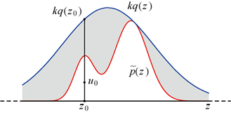
• Reject samples in the gray region ($u_0 > \tilde{p}(z_0)$).
• Limitation: In high-dimensional spaces, $k$ is typically very large and the acceptance rate is extremely low (decreasing exponentially), so practical utility is limited. Imagine that in a 100-dimensional space, a rectangular box that “just encloses” the target region has the vast majority of its volume outside the target region.

Adaptive Rejection Sampling

Intuition: The problem with rejection sampling is that “the rectangle encloses too much, wasting too many points”. The idea of adaptive rejection sampling is: start with a coarse envelope, and each time a sample is rejected, add the information at that location, making the envelope fit tighter and tighter — like continually pruning the branches and leaves of a tree so that it conforms more and more closely to the target shape.

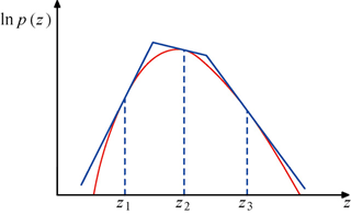
• Improvement: For Log-Concave Distributions (i.e., $\ln p(z)$ has the shape of an upside-down bowl), dynamically construct an Envelope Function (the “lid” on top):
  1. Compute $\ln p(z)$ and its gradient at initial grid points, and use tangent lines to construct a piecewise exponential envelope function.
  2. Sample from the envelope function; if a sample is rejected, add it to the grid points and update the envelope function.
• Advantage: No need to manually choose $q(z)$; the envelope is optimized over iterations, reducing the rejection rate.

Importance Sampling

Intuition: You cannot sample from the target distribution $p(z)$, but you can sample from another “similar” distribution $q(z)$. What to do? You sample from $q(z)$ and then “score” each sample — if a sample has high probability under $p(z)$ but low probability under $q(z)$, you assign it a higher weight; otherwise you lower its weight. This is Importance Sampling: using weights to correct for the difference between distributions.

• Goal: Estimate $\mathbb{E}[f] = \int f(z) p(z) dz$, but cannot sample directly from $p(z)$.
• Method: Sample from the proposal distribution $q(z)$, and correct the bias using Importance Weights: $$\mathbb{E}[f] = \int f(z) \frac{p(z)}{q(z)} q(z) dz \simeq \frac{1}{L} \sum_{l=1}^L \frac{p(z^{(l)})}{q(z^{(l)})} f(z^{(l)})$$ where $r_l = \frac{p(z^{(l)})}{q(z^{(l)})}$ is called the importance weight.
• Unnormalized distributions: If $p(z) = \tilde{p}(z)/Z_p$ and $q(z) = \tilde{q}(z)/Z_q$, then: $$\mathbb{E}[f] \simeq \sum_{l=1}^L w_l f(z^{(l)}), \quad w_l = \frac{\tilde{p}(z^{(l)}/q(z^{(l)})}{\sum_m \tilde{p}(z^{(m)}/q(z^{(m)})}$$
• Limitation: If $q(z)$ differs greatly from $p(z)$, the weights may concentrate on a few samples, the effective sample size is low, and the error cannot be diagnosed.

Sampling-Importance-Resampling (SIR)

Intuition: First use importance sampling to score the samples, then resample once based on the scores — samples with high scores are more likely to be selected, while those with low scores are naturally eliminated. Like a talent show: first hold auditions and score, then decide who advances based on the scores.

• Steps:
  1. Sample $L$ samples from $q(z)$ and compute the weights $w_l$.
  2. Resample $L$ samples from these, where the probability of each sample being selected is proportional to $w_l$.
• Advantage: No need to determine $k$ as in rejection sampling; after resampling, the samples approximately follow $p(z)$ (exact when $L \to \infty$).

Markov Chain Monte Carlo Sampling {#mcmc}

Intuition: Imagine a drunk person walking around a city. The direction of each step is random, but with a peculiar property — he walks slowly (stays longer) where there are many people, and walks fast where there are few. After walking long enough, the frequency with which he appears at various places will be proportional to the population density. This is the core idea of Markov Chain Monte Carlo (MCMC): build a “chain” of random walks such that its eventual “stationary distribution” is exactly the target distribution we want to sample from.

• Core idea: Construct a Markov Chain (a random process where “the next step depends only on the current position”) such that its Stationary Distribution (the stable distribution reached after the chain has run for a long time) is the target distribution $p(z)$, and generate samples through iterations of the chain.

Markov Chain Basics

Where you go next depends only on your current position, not on the path you took before — this is the Markov Property (also called “memorylessness”).

• Definition: A Random Variable Sequence $z^{(1)}, z^{(2)}, ...$ satisfying $p(z^{(m+1)} | z^{(1)}, ..., z^{(m)}) = p^{(m+1)} | z^{(m)})$ , whose Transition Probability is $T(z', z) = p(z | z')$ — representing “the probability of jumping from $z'$ to $z$”.
• Stationary Distribution: After a long time, the system reaches an equilibrium state, and the proportion of each state no longer changes. Mathematically: if $p^*(z) = \int T(z', z) p^*(z') dz'$, then $p^*(z)$ is the stationary distribution.
• Detailed Balance: The “flow” from state A to state B equals the “flow” from state B to state A. If $p^*(z) T(z, z') = p^*(z') T(z', z)$, then $p^*(z)$ is a stationary distribution (a reversible chain).
• Ergodicity: The chain converges to a unique stationary distribution, independent of the initial distribution, ensuring that the samples eventually follow $p(z)$.

Metropolis Algorithm

Intuition: The rule for the drunk person’s walk is simple — starting from the current position, randomly pick a nearby location as a candidate. If the candidate is “better” (higher target probability), walk there; if “worse”, flip a coin, with the probability proportional to the ratio of the old and new positions’ probabilities. This ensures the drunk person stays longer in high-probability regions.

• Steps:
  1. Initial state $z^{(0)}$, iteratively generate a Candidate Sample $z^* \sim q(z | z^{(\tau)})$ (a Symmetric Proposal, i.e., $q(z_A | z_B) = q(z_B | z_A)$).
  2. Acceptance Probability: $A(z^*, z^{(\tau)}) = \min(1, \frac{\tilde{p}(z^*)}{\tilde{p}(z^{(\tau)})})$.
  3. If $u \sim U(0,1) < A$, then $z^{(\tau+1)} = z^*$ (accept, walk to the new position); otherwise $z^{(\tau+1)} = z^{(\tau)}$ (reject, stay in place).
• Property: Under a symmetric proposal distribution, detailed balance is satisfied, and the stationary distribution is $p(z)$.
• Limitation: Samples may be highly correlated (adjacent samples may be identical), so Thinning (e.g., keeping every $M$-th sample) is needed to approximate independence.

Metropolis-Hastings Algorithm

Intuition: The Metropolis algorithm requires the proposal distribution to be symmetric (the probability of going left and right is the same), but in reality we may need an asymmetric proposal. The Metropolis-Hastings algorithm compensates for this asymmetry by adding a “correction factor” to the acceptance probability — like adding a counterweight to a balance scale to restore equilibrium.

• Improvement: Relax the symmetry requirement on the proposal distribution; the acceptance probability is adjusted to: $$A(z^*, z^{(\tau)}) = \min\left(1, \frac{\tilde{p}(z^*) q(z^{(\tau)} | z^*)}{\tilde{p}(z^{(\tau)}) q(z^* | z^{(\tau)})}\right)$$ The extra $\frac{q(z^{(\tau)} | z^*)}{q(z^* | z^{(\tau)})}$ is the correction factor, compensating for the asymmetry of the proposal distribution.
• Advantage: Applicable to a broader range of proposal distributions, still satisfies detailed balance.
• Challenge: The choice of proposal distribution affects efficiency — if the variance is too small, the random walk is slow (the drunk person shuffles in place); if too large, the rejection rate is high (the drunk person keeps getting bounced back).

Gibbs Sampling

Intuition: Imagine you are adjusting an audio system with many knobs. The strategy of Gibbs Sampling is: each time, turn only one knob, keeping all the other knobs fixed, and decide where that knob should be turned based on the conditional probability. By adjusting each knob in turn, the audio system will eventually reach its optimal state. By moving only one dimension at a time, the difficulty of sampling is greatly simplified.

• Applicable scenario: High-dimensional distribution $p(z_1, ..., z_M)$, where it is convenient to sample the Conditional Distribution $p(z_i | z_{\backslash i})$ ($z_{\backslash i}$ being all variables except $z_i$).
• Steps:
  1. Initialize $z^{(0)} = (z_1^{(0)}, ..., z_M^{(0)})$.
  2. Iteratively update each variable: $z_i^{(\tau+1)} \sim p(z_i | z_1^{(\tau+1)}, ..., z_{i-1}^{(\tau+1)}, z_{i+1}^{(\tau)}, ..., z_M^{(\tau)})$.
• Principle: Each update satisfies detailed balance, the stationary distribution is $p(z)$, and the acceptance rate is 1 (it is a special case of Metropolis-Hastings — all candidate points are accepted).
• Improvements: Block Gibbs Sampling (updating a group of variables simultaneously) reduces correlation; Over-relaxation accelerates convergence.

Ancestral Sampling

Height ← parents’ average height + random factors — this “cause-to-effect” sampling method is Ancestral Sampling.

• Applicable scenario: Directed Graphical Model (a probabilistic graphical model that uses arrows to represent causal relationships, with no observed variables), with joint distribution $p(z) = \prod p(z_i | \text{pa}(i))$ (where $\text{pa}(i)$ is the Parent Node).
• Steps: Sample in Topological Order (i.e., the order from “ancestors” to “descendants”); each variable is sampled from its conditional distribution $p(z_i | \text{pa}(i))$ (the parent nodes are already determined).
• Extension: Likelihood Weighted Sampling (handling observed variables), which assigns weights $\prod p(z_i | \text{pa}(i))$ to the observed variables.

Langevin Sampling

Energy-Based Models

Intuition: Imagine a topographic map — valleys (low-energy regions) correspond to high-probability regions, and peaks (high-energy regions) correspond to low-probability regions. An Energy-Based Model uses an “energy function” to define a probability distribution: the lower the energy at a location, the higher the probability.

• Definition: Define the distribution through an Energy Function $E(x, w)$: $$p(x | w) = \frac{1}{Z(w)} e^{-E(x, w)}, \quad Z(w) = \int e^{-E(x, w)} dx$$ where $Z(w)$ is the Partition Function (i.e., the normalization constant, usually difficult to compute — it requires integrating over the entire space).
• Training challenge: The likelihood function depends on $Z(w)$, so the gradient must be approximated.

Likelihood Maximization

Intuition: Training an energy-based model is like adjusting the terrain — “dig down” (lower the energy, increase the probability) where real data appears, and “pile up” (raise the energy, lower the probability) where the model generates incorrectly.

• Gradient formula: $$\nabla_w \mathbb{E}_{x \sim p_D}[\ln p(x | w)] = -\mathbb{E}_{x \sim p_D}[\nabla_w E(x, w)] + \mathbb{E}_{x \sim p_M}[\nabla_w E(x, w)]$$ where $p_D$ is the Data Distribution (the probability distribution of the real data), and $p_M$ is the Model Distribution (the probability distribution defined by the model).

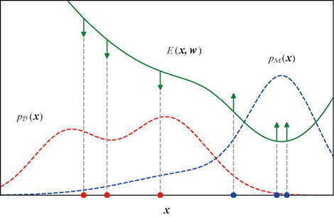
The energy function E(x, w) (green) and the associated model distribution pM(x) and true data distribution pD(x). Using the above equation to increase the expected log-likelihood pushes up the energy function at points corresponding to model samples (shown as blue dots), and pulls down the energy function at points corresponding to data set samples (shown as red dots).

Langevin Dynamics (Sampling Process)

Intuition: Imagine a small ball rolling on an energy landscape. It slides down (in the gradient direction), while subject to random perturbations (like the molecular collisions in Brownian motion). This way the ball will eventually concentrate in the valleys (high-probability regions), and will not get stuck at some local minimum. This is Langevin Dynamics — using gradient information to guide sampling, while adding random noise to avoid getting trapped in local optima.

• Principle: Use gradient information to guide sampling; the update formula is: $$x^{(\tau+1)} = x^{(\tau)} + \eta \nabla_x \ln p(x^{(\tau)}, w) + \sqrt{2\eta} \epsilon^{(\tau)}$$ where $\epsilon^{(\tau)} \sim \mathcal{N}(0, I)$, $\eta$ is the Step Size, and $\nabla_x \ln p(x, w) = -\nabla_x E(x, w)$ (the Score Function, i.e., the gradient of the log-probability).
• Property: As $\eta \to 0$ and with sufficiently many iterations, the samples converge to $p(x | w)$.
• Contrastive Divergence: Use short-chain sampling (running only a few steps, e.g., 1 step) to approximate the model distribution, reducing computational cost, suitable for energy adjustment in the neighborhood of the data. It is like you don’t need to let the ball roll all the way to the bottom of the valley; you just need to let it slide down a short distance to roughly know the direction.

Chapter 14 Summary

One-sentence version: Sampling is “drawing lots” from a probability distribution — for simple distributions draw directly; for complex ones use various tricks (transform, reject, weight, random walk) to draw.

Knowledge map:

1
Sampling Methods
2
├── Basic Sampling
3
│   ├── Inverse Transform: use the inverse of the CDF to morph a uniform random number
4
│   ├── Box-Muller: specifically generates Gaussian samples
5
│   ├── Rejection Sampling: scatter points in a large box, keep those within the target region
6
│   ├── Importance Sampling: sample from a stand-in distribution, correct bias with weights
7
│   └── SIR: Importance Sampling + Resampling
8
├── MCMC Methods
9
│   ├── Metropolis: drunk person's walk, symmetric proposal
10
│   ├── Metropolis-Hastings: drunk person's walk, asymmetric proposal
11
│   └── Gibbs Sampling: adjust only one knob at a time
12
└── Langevin Sampling
13
    ├── Energy-Based Model: define probability with an energy function
14
    └── Langevin Dynamics: ball rolls down the gradient + random perturbation

Chapter 15 Discrete Latent Variables {#discrete-latent}

Intuition: You see a person’s behavior (observed variable), but you cannot see their inner emotions (latent variable). Although emotions are invisible, they profoundly influence behavior. Introducing “latent variables” lets the model learn to “guess” these hidden factors.

In probabilistic models, we typically encounter two kinds of variables: Observed Variables (such as images, numerical values, etc. in a dataset — things we can directly see) and Latent Variables (Latent Variable, also called Hidden Variable — variables we cannot see but that are important for modeling). For the basics of probability distributions, please refer to Part 1 notes.

Discrete Latent Variables are latent variables that take discrete values (such as “yes/no”, “category 1/category 2/category 3”). There are mainly two reasons to introduce them:

• Some latent variables correspond to real but unobserved quantities (for example, in an animal image, the animal’s “orientation” is a latent variable — we did not observe it directly, but it affects the pixel distribution of the image);
• Even when there is no real corresponding quantity, introducing latent variables makes the model more flexible — by constructing the Joint Distribution (Joint Distribution, i.e., the probability of all variables together) of “observed variables + latent variables”, we simplify the complex Marginal Distribution (Marginal Distribution, i.e., the observed variable distribution obtained by summing over all possible values of the latent variables) of the observed variables.

K-means Clustering

Intuition: As the saying goes, “birds of a feather flock together”. Given a bunch of mixed fruits, you would naturally put the apples in one pile and the oranges in another — this is Clustering. K-means is the simplest clustering method: first randomly select K “centers”, then assign each data point to the nearest center, then update the center positions, and iterate until stable.

K-means (K-means algorithm) is a clustering algorithm whose goal is to divide N D-dimensional data points (such as 2D coordinate points, 3D RGB pixels) into K “clusters”. Points in the same cluster should be close, and points in different clusters should be far apart.

Assume each cluster has a “center” (denoted by $\mu_k$ for the center of the k-th cluster). We measure the quality of the clustering using the sum of squared distances from each data point to the center of its assigned cluster, and the smaller this value the better.

To express “which cluster a data point belongs to”, we introduce the Indicator Variable (Indicator Variable, a 0/1 marker) $r_{nk}$:

• If the n-th data point belongs to the k-th cluster, $r_{nk}=1$;
• Otherwise, $r_{nk}=0$ (each data point belongs to only one cluster, so for each n, only one $r_{nk}=1$).

Thus, the “sum of squared distances” can be written as:

Our goal is to find the optimal $r_{nk}$ and $\mu_k$ that minimize J.

K-means optimizes J by repeatedly iterating the following two steps until the result stops changing:

1. E-step (Assignment step): Fix the cluster centers $\mu_k$, and find the nearest cluster for each data point. For each data point $x_n$, compute its distance to all cluster centers, and assign it to the cluster that is nearest, i.e.:

   $$r_{nk} = \begin{cases}1 & \text{if } k \text{ is the cluster center nearest to } x_n \\ 0 & \text{otherwise}\end{cases}$$

   For example, suppose data point $x_1$ is at distance 2 from $\mu_1$ and distance 5 from $\mu_2$, then $r_{11}=1$, $r_{12}=0$.

2. M-step (Update step): Fix the assignments $r_{nk}$, and recompute the cluster centers. The new center of each cluster is the “average” (mean) of all data points in that cluster:

   $$\mu_k = \frac{\sum_{n=1}^N r_{nk} x_n}{\sum_{n=1}^N r_{nk}}$$

   For example, if the 1st cluster has 3 data points $x_2, x_5, x_7$, then $\mu_1 = (x_2 + x_5 + x_7)/3$.

Example

Using data from the Old Faithful geyser in Yellowstone National Park (each data point has two features: eruption duration and waiting time until the next eruption). When K=2 — it is like dividing the geyser into two categories: “long eruption, long wait” and “short eruption, short wait”:

• Initially, randomly pick two points as $\mu_1$ and $\mu_2$;
• E-step: each data point is assigned to the cluster of the nearest center (equivalent to drawing a perpendicular bisector, with the two sides belonging to two clusters);
• M-step: based on the assignment results, compute the new centers of the two clusters (e.g., the average of all points in the left cluster);
• Repeat the above steps until the cluster centers no longer change (convergence).

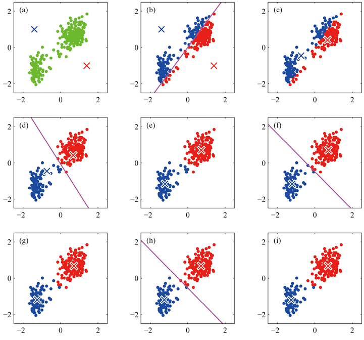
K-means algorithm for Yellowstone National Park

• K-means is guaranteed to converge within a finite number of steps (since the assignment method is finite, and J only decreases or stays the same at each iteration), but it may converge to a “local optimum” (not the best clustering result), so it is common to try several different initial centers.
• The K must be specified in advance (e.g., by experience or other methods).

Gaussian Mixture Distribution

Intuition: K-means is “hard clustering” — each point belongs to only one cluster, black or white. But in reality some points may be “ambiguous”; for example, a point in the middle of two clusters is hard to say it fully belongs to either. The Gaussian Mixture Model (GMM) solves this with “soft clustering” (Soft Clustering, where each point belongs to different clusters with a certain probability) — like saying “this fruit is 70% like an apple and 30% like a pear”.

GMM assumes the observed data is “mixed” from K Gaussian distributions (i.e., normal distributions, detailed in Part 2 notes):

• First choose one of the K Gaussian distributions (the probability of choosing the k-th is $\pi_k$, where $\pi_k$ is called the Mixing Coefficient, i.e., the “weight” of each Gaussian component), satisfying $\sum \pi_k=1$;
• Then generate a data point from the selected Gaussian distribution.

So, the probability distribution of data x is:

where $\mathcal{N}(x | \mu_k, \Sigma_k)$ is the k-th Gaussian distribution (mean $\mu_k$, covariance $\Sigma_k$, see the Gaussian distribution introduction in Part 2 notes).

Introduce the discrete latent variable z (1-of-K encoding):

• Probability of the latent variable: $p(z_k=1) = \pi_k$ (the probability of choosing the k-th Gaussian);
• Given z=k, the probability of x: $p(x | z_k=1) = \mathcal{N}(x | \mu_k, \Sigma_k)$.

Thus, the joint distribution of x and z is $p(x,z) = p(z)p(x|z)$, and the GMM distribution is the marginal distribution summing over z: $p(x) = \sum_z p(x,z)$.

For a data point x, its Posterior Probability (Posterior Probability, i.e., the probability of inferring the cause after knowing the result x) of coming from the k-th Gaussian is called the “Responsibility” (Responsibility), denoted $\gamma(z_k)$ — which can be understood as “the contribution of the k-th Gaussian to this data point”:

For example, if x has a 70% probability of coming from the 1st Gaussian and 30% from the 2nd, then $\gamma(z_1)=0.7$, $\gamma(z_2)=0.3$, which is “soft assignment”.

The parameters of GMM are $\pi_k$, $\mu_k$, $\Sigma_k$, which need to be estimated from the data. Since the probability formula contains a sum inside a logarithm ($\ln \sum \pi_k \mathcal{N}(...)$ ), directly maximizing it is troublesome, and this is when the EM algorithm is needed.

EM Algorithm {#em-algorithm}

Intuition: Imagine you are looking for the deepest pit in a dark room. You cannot see where the pit is (the latent variable is unknown), but you can:

1. Guess — based on the slope of the ground beneath your feet, guess roughly which direction the pit is in (E-step);
2. Take a step — walk one step in that direction (M-step);
3. Repeat — at the new position, guess again, walk again, until you can no longer move (convergence).

This is the core of the EM Algorithm (Expectation-Maximization Algorithm) — a “guess-verify-improve” loop.

The EM algorithm is a general method for handling models with latent variables. Its core idea is: by “guessing” the values of the latent variables (E-step), then using the guessed values to estimate the parameters (M-step), and iterating until the parameters stabilize.

Suppose we have observed data X and latent variables Z, with model parameters $\theta$, and the goal is to maximize the Likelihood (Likelihood, i.e., the probability of the observed data under the model parameters) $p(X | \theta)$.

1. E-step (Expectation step): Compute the “expectation of the complete-data log-likelihood”. The complete data is (X,Z), but Z is unknown, so we use the current parameters $\theta^{old}$ to compute the posterior distribution of Z $p(Z | X, \theta^{old})$ , then compute the expectation of the complete-data log-likelihood (called the Q function):

   $$\mathcal{Q}(\theta, \theta^{old}) = \sum_Z p(Z | X, \theta^{old}) \ln p(X,Z | \theta)$$

   where $\sum_Z$ is the sum over all possible values of the latent variable $Z$, $p(Z | X, \theta^{old})$ is the latent variable posterior computed with the old parameters (“the guess in the E-step”), and $\ln p(X,Z | \theta)$ is the complete-data log-likelihood. In short: the Q function is a score of “how good the new parameters $\theta$ are, under the guess of the old parameters”.

2. M-step (Maximization step): Maximize the Q function to get the new parameters. Find $\theta^{new}$ that maximizes $\mathcal{Q}(\theta, \theta^{old})$:

   $$\theta^{new} = \arg\max_\theta \mathcal{Q}(\theta, \theta^{old})$$

Repeat the above two steps until the parameters no longer change.

EM Applied to GMM

For GMM, the parameters are $\theta = \{\pi_k, \mu_k, \Sigma_k\}$, and the EM steps are:

• E-step: Compute the responsibility $\gamma(z_{nk})$ of each data point $x_n$ for each cluster k (using the responsibility formula above);
• M-step: Update the parameters using the responsibilities:
  • Effective point count: $N_k = \sum_{n=1}^N \gamma(z_{nk})$ (the responsibilities of each point summed up, similar to “weighted counting”);
  • Mean: $\mu_k = \frac{1}{N_k} \sum_{n=1}^N \gamma(z_{nk}) x_n$ (weighted average);
  • Covariance: $\Sigma_k = \frac{1}{N_k} \sum_{n=1}^N \gamma(z_{nk}) (x_n - \mu_k)(x_n - \mu_k)^T$ (weighted variance);
  • Mixing coefficient: $\pi_k = \frac{N_k}{N}$ (the proportion of effective points to total points).

The EM algorithm guarantees that after each iteration, the likelihood $p(X | \theta)$ will not decrease (it can only increase or stay the same), so it will eventually converge to a local optimum.

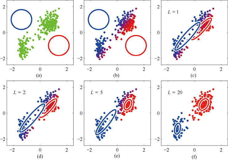
EM algorithm for Yellowstone National Park

Evidence Lower Bound

The Evidence Lower Bound ELBO (Evidence Lower Bound) is a mathematical tool that helps us understand why the EM algorithm works, and can be extended to more complex models (such as variational autoencoders). Its core idea is: directly optimizing the likelihood is difficult (because of the sum/integral over latent variables), but we can optimize a “lower bound” of the likelihood — an easier-to-compute surrogate objective.

Decomposition of the Likelihood

For any distribution $q(Z)$ (which can be any distribution we choose about the latent variable Z), the log-likelihood of the observed data can be decomposed as:

where:

• $\mathcal{L}(q, \theta)$ is the ELBO, with the formula: $\mathcal{L}(q, \theta) = \sum_Z q(Z) \ln \left( \frac{p(X,Z | \theta)}{q(Z)} \right)$;
• $KL(q \| p)$ is the Kullback-Leibler Divergence (KL Divergence, a measure of the difference between two distributions, which can be understood as “the extra amount of information wasted when using distribution q to encode distribution p”), and $KL(q \| p) \ge 0$ (equal to 0 if and only if $q(Z) = p(Z | X, \theta)$).

Since $KL(q \| p) \ge 0$, we have $\mathcal{L}(q, \theta) \le \ln p(X | \theta)$, i.e., the ELBO is a “lower bound” of the log-likelihood.

The EM algorithm is in fact optimizing this lower bound:

• E-step: choose $q(Z) = p(Z | X, \theta^{old})$, at which point $KL=0$ and the ELBO equals the current likelihood;
• M-step: fix q, maximize the ELBO to obtain $\theta^{new}$, at which point the likelihood also increases (because the lower bound is raised).

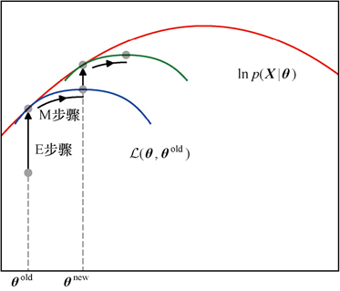
The EM algorithm computes the lower bound of the log-likelihood at the current parameter values, then maximizes this lower bound to obtain new parameter values.

Chapter 15 Summary

One-sentence version: Discrete latent variable models are “guessing hidden causes” — K-means guesses with hard classification, GMM guesses with soft probabilities, and the EM algorithm provides a general “guess-improve” iterative framework.

Knowledge map:

1
Discrete Latent Variables
2
├── K-means Clustering (hard clustering)
3
│   ├── E-step: assign each point to the nearest cluster
4
│   └── M-step: update cluster center to the mean
5
├── Gaussian Mixture Model GMM (soft clustering)
6
│   ├── each point belongs to different clusters with a probability (responsibility)
7
│   └── learn parameters with the EM algorithm
8
├── EM Algorithm (general framework)
9
│   ├── E-step: compute the Q function (expectation of the latent variable posterior)
10
│   └── M-step: maximize the Q function to update parameters
11
└── Evidence Lower Bound ELBO
12
    ├── log-likelihood = ELBO + KL divergence
13
    └── the EM algorithm is optimizing the ELBO

These methods are widely used in tasks such as clustering, classification, and density estimation. For the basics of classification tasks, please refer to Part 3 notes.

Chapter 16 Continuous Latent Variables {#continuous-latent}

Many datasets have the characteristic that although the data points are located in a high-dimensional space, they actually lie on a low-dimensional Manifold (i.e., a curved low-dimensional surface, see Chapter 6 - Data Manifold ). The latent degrees of freedom that control the variation of the data are the Continuous Latent Variables.

Intuition: Imagine a 3D object illuminated by light; its shadow on the wall is 2D. Although the shadow loses some information, it retains the most important shape features of the object. Continuous latent variable models do something similar — find the most important “shadow” (low-dimensional representation) of the data, and discard unimportant details.

Continuous latent variable models can effectively model such data by first selecting points in the latent variable space (low-dimensional) and then adding noise to generate the observed data. This chapter starts with the classic Principal Component Analysis (PCA), and gradually introduces continuous latent variable models such as probabilistic PCA and factor analysis.

Principal Component Analysis PCA

Intuition: PCA is like “shadow projection” — you have a 3D object (high-dimensional data), and want to find a wall (low-dimensional subspace) such that the object’s shadow (projection) preserves the object’s shape information as much as possible. The key question is: which direction should the wall face? PCA’s answer is: face the direction of maximum data variation. Imagine standing in front of a scattered group of points taking a photo — if you shoot from the front (the direction of maximum data variation), you can best distinguish the points; if you shoot from the side (the direction of small variation), many points will overlap.

PCA (Principal Component Analysis) is a commonly used Linear Dimensionality Reduction method (i.e., using a linear transformation to map high-dimensional data to low dimensions). Its core is to project high-dimensional data onto a low-dimensional linear subspace (Principal Component Space) while preserving the main information of the data.

Maximum Variance Formulation

One definition of PCA is: find a low-dimensional subspace such that the Variance (Variance, a measure of how spread out the data is; the larger it is, the more “spread out” the data) of the data projected onto that subspace is maximized (i.e., retaining the most information).

• Data preprocessing: First compute the data Mean (Mean, i.e., the average) $\overline{x}$, and Center the data (Centering, i.e., subtract the mean so that the data is centered at the origin):

  $$\overline{x} = \frac{1}{N}\sum_{n=1}^N x_n$$

  where $x_n$ is a D-dimensional data point and $N$ is the number of samples.

• Projection variance: For a 1-dimensional principal component ($M=1$), use a unit vector $u_1$ to represent the projection direction. The projection value of data point $x_n$ is $u_1^T x_n$, and the variance after projection is:

  $$\frac{1}{N}\sum_{n=1}^N (u_1^T x_n - u_1^T \overline{x})^2 = u_1^T S u_1$$

  where $S$ is the data Covariance Matrix (Covariance Matrix, a square matrix describing the correlation between the dimensions of the data; the diagonal is the variance of each dimension):

  $$S = \frac{1}{N}\sum_{n=1}^N (x_n - \overline{x})(x_n - \overline{x})^T$$

• Optimize the projection direction: Maximize the variance under the constraint $u_1^T u_1 = 1$ (unit vector constraint); via the method of Lagrange multipliers we get:

  $$S u_1 = \lambda_1 u_1$$

  i.e., $u_1$ is an Eigenvector of $S$ (Eigenvector, i.e., a vector whose direction is unchanged under the action of the matrix), and $\lambda_1$ is the corresponding Eigenvalue (Eigenvalue, i.e., the factor by which the eigenvector is stretched). The maximum variance corresponds to the eigenvector of the largest eigenvalue (First Principal Component).

• High-dimensional principal components: For an M-dimensional principal component space, the optimal projection directions are the eigenvectors $u_1, u_2, ..., u_M$ corresponding to the first $M$ largest eigenvalues of the covariance matrix $S$.

Minimum Error Formulation

Another equivalent definition of PCA is: find a low-dimensional subspace such that the average squared distance from the data points to their projections (Projection Error) is minimized. “Maximum variance” and “minimum error” are two sides of the same coin — the larger the projection variance, the less information is lost, and the smaller the error.

• Projection error: Use $M$ orthogonal basis vectors $u_1, ..., u_M$ to span the principal component space. The projection of data point $x_n$ is $\tilde{x}_n$, and the error is:

  $$J = \frac{1}{N}\sum_{n=1}^N \|x_n - \tilde{x}_n\|^2$$

• Optimal projection: By derivation, the minimum error corresponds to choosing the eigenvectors of the first $M$ largest eigenvalues of the covariance matrix $S$ as the basis vectors, in which case the error is:

  $$J = \sum_{i=M+1}^D \lambda_i$$

  i.e., the error equals the sum of the discarded eigenvalues.

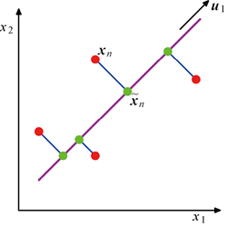
The principal subspace is shown with magenta lines. PCA causes the orthogonal projections of the data points (red points) onto the principal subspace to maximize the variance of the projected points (green points). The errors are shown with blue lines.

Data Compression

PCA can be used for data compression: project D-dimensional data $x_n$ onto the M-dimensional principal component space, and represent the data using projection coefficients.

• Reconstruct data: The compressed data can be reconstructed via the projection coefficients: $\tilde{x}_n = \overline{x} + \sum_{i=1}^M (x_n^T u_i - \overline{x}^T u_i) u_i$ where $(x_n^T u_i - \overline{x}^T u_i)$ is the M-dimensional projection coefficient.

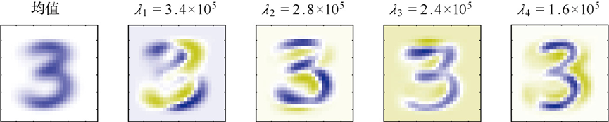
The mean vector and the first 4 PCA eigenvectors with their corresponding eigenvalues

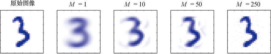
A handwritten digit and its PCA reconstruction obtained by retaining M principal components. As the value of M increases, the reconstruction becomes more accurate.

Data Whitening

Whitening is a data preprocessing that transforms the data into a form with zero mean, unit covariance, and uncorrelated dimensions — like “kneading” a cloud of arbitrary shape into a standard sphere. Whitened data is easier for machine learning algorithms to process.

• Whitening steps:
  1. Center the data (subtract the mean);
  2. Compute the eigenvalues $\lambda_i$ and eigenvectors $u_i$ of the covariance matrix $S$;
  3. Transform the data: $$y_n = L^{-1/2} U^T (x_n - \overline{x})$$ where $U$ is the eigenvector matrix and $L$ is the diagonal eigenvalue matrix. The covariance of the transformed data is the identity matrix.

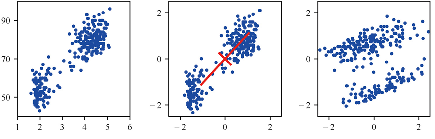
Whitened data, with mean 0 and covariance equal to the identity matrix

High-Dimensional Data Handling

When the data dimension $D$ is much larger than the number of samples $N$, directly computing the covariance matrix $S$ ($D×D$) is costly. In this case, it can be simplified via low-dimensional matrix operations:

• Define the centered data matrix $X$ ($N×D$, each row is $x_n - \overline{x}$), then $S = N^{-1} X^T X$;
• Compute the eigenvalues and eigenvectors of $X X^T$ ($N×N$) to indirectly obtain the eigenvalues and eigenvectors of $S$, reducing the computational cost from $O(D^3)$ to $O(N^3)$.

Probabilistic Latent Variables

Traditional PCA is Deterministic (Deterministic, i.e., given the data, the result is unique), while Probabilistic PCA generalizes it into a Probabilistic Model (Probabilistic Model, i.e., using a probability distribution to describe uncertainty), which is more flexible and facilitates handling missing data, performing Bayesian Inference (Bayesian Inference, i.e., expressing uncertainty with probability and updating beliefs based on new data), etc.

Generative Model

Probabilistic PCA assumes the data is generated by a “latent variable → observed variable” generative process:

• Latent variable: An M-dimensional latent variable $z \sim \mathcal{N}(z | 0, I)$ (zero-mean, unit-covariance Gaussian);
• Observed variable: Given $z$, the D-dimensional observed variable $x \sim \mathcal{N}(x | W z + \mu, \sigma^2 I)$, where $W$ is the $D×M$ mapping matrix, $\mu$ is the mean, and $\sigma^2$ is the noise variance.

The generative process can be written as: $x = W z + \mu + \epsilon$, where $\epsilon \sim \mathcal{N}(0, \sigma^2 I)$ is the noise (Figure 16.7 shows an intuitive illustration of this generative process).

Likelihood Function

The marginal distribution $p(x)$ (integrating over $z$) is still a Gaussian distribution: $p(x) = \mathcal{N}(x | \mu, C)$ where the covariance matrix $C = W W^T + \sigma^2 I$.

• Log-likelihood: Given a dataset $X = \{x_n\}$, the log-likelihood is:

  $$\ln p(X | \mu, W, \sigma^2) = -\frac{ND}{2}\ln(2\pi) - \frac{N}{2}\ln|C| - \frac{1}{2}\sum_{n=1}^N (x_n - \mu)^T C^{-1} (x_n - \mu)$$

• Posterior distribution: Given $x$, the posterior distribution of the latent variable $z$ is also Gaussian:

  $$p(z | x) = \mathcal{N}(z | M^{-1} W^T (x - \mu), \sigma^2 M^{-1})$$

  where $M = W^T W + \sigma^2 I$ (Figure 16.8 shows the graphical model structure of probabilistic PCA).

Maximum Likelihood Estimation

Solve the parameters by maximizing the log-likelihood:

• Mean $\mu$: The optimal solution is the data mean $\mu = \overline{x}$;
• Mapping matrix $W$: The maximum likelihood solution is $W_{ML} = U_M (L_M - \sigma^2 I)^{1/2} R$, where $U_M$ is the first $M$ eigenvectors of $S$, $L_M$ is the corresponding eigenvalues, and $R$ is an orthogonal matrix (rotation of the latent space);
• Noise variance $\sigma^2$: The optimal solution is the average of the discarded eigenvalues: $$\sigma_{ML}^2 = \frac{1}{D - M}\sum_{i=M+1}^D \lambda_i$$

Factor Analysis

Factor Analysis is similar to probabilistic PCA, but the conditional covariance of the observed variables is a Diagonal Matrix (Diagonal Matrix, i.e., only the diagonal has values, the noise of each dimension is independent but can differ), rather than isotropic (same noise in all directions):

• Conditional distribution: $p(x | z) = \mathcal{N}(x | W z + \mu, \Psi)$, where $\Psi$ is a diagonal matrix (independent noise per dimension);
• Marginal covariance: $C = W W^T + \Psi$, modeling the noise of different dimensions more flexibly.

Independent Component Analysis ICA

Independent Component Analysis (ICA) assumes that the latent variables are Statistically Independent (Statistically Independent, i.e., the information of one variable cannot help infer another) non-Gaussian variables, used for problems such as Blind Source Separation (Blind Source Separation, e.g., separating individual speakers from a mixture of sounds):

• Latent variable distribution: $p(z) = \prod_{j=1}^M p(z_j)$ (factorized, non-Gaussian);
• Observed variable: $x = W z + \mu$ (no noise, or low noise). By maximizing the likelihood, independent sources can be separated from the mixed signal (e.g., separating mixed speech signals).

Kalman Filter

The Kalman Filter is used for Sequential Data (Sequential Data, such as time series), where the latent variables form a Markov Chain (i.e., each moment’s latent variable depends only on the previous moment):

• Latent variable: $z_n \sim p(z_n | z_{n-1})$ (Gaussian, with mean a linear function of $z_{n-1}$);
• Observed variable: $x_n \sim \mathcal{N}(x_n | W z_n + \mu, \sigma^2 I)$. Suitable for real-time tracking (e.g., radar tracking of aircraft).

Evidence Lower Bound ELBO

Similar to discrete latent variables, the log-likelihood of continuous latent variable models can be decomposed into the sum of the ELBO and the KL divergence (this decomposition was introduced in Chapter 15):

• ELBO:

  $$\mathcal{L}(q, w) = \int q(z) \ln\left( \frac{p(x, z | w)}{q(z)} \right) dz$$ $$\mathcal{KL}(q, w) = - \int q(z) \ln\left( \frac{p(z| x , w)}{q(z)} \right) dz$$

  which is a lower bound of the log-likelihood (since $KL \geq 0$).

• Significance: The ELBO is the core of Variational Inference (Variational Inference, a technique that uses optimization methods to approximate inference). By optimizing $q(z)$ and the model parameters $w$, we can indirectly maximize the log-likelihood.

EM Algorithm for Probabilistic PCA

Probabilistic PCA can also use the EM algorithm to learn parameters. Intuitively: the E-step guesses each data point’s “hidden coordinates” (latent variable z), and the M-step updates the mapping matrix W based on these guesses. Below is the complete formula derivation — if you only care about intuition, you can skip the formula part.

Advantages of the EM Algorithm

Compared to traditional PCA based on Eigendecomposition (Eigendecomposition, i.e., decomposing a matrix into eigenvectors and eigenvalues), the EM algorithm has significant computational advantages when handling large-scale data.

• Computational complexity of traditional PCA: First compute the data covariance matrix $\mathbf{S} = \frac{1}{N}\sum_{n=1}^N (\mathbf{x}_n - \bar{\mathbf{x}})(\mathbf{x}_n - \bar{\mathbf{x}})^T$ , with complexity $O(ND^2)$.

  • Then perform eigendecomposition on the $D \times D$ covariance matrix, with complexity $O(D^3)$.
  • If only the first $M$ principal components are computed, more efficient algorithms (such as power iteration) can be used, with complexity about $O(MD^2)$, but the $O(ND^2)$ for computing the covariance matrix remains the bottleneck.

• Computational complexity of the EM algorithm:

  • The most time-consuming operations in the E-step and M-step are traversing all data points and computing the sums, e.g., $\sum_{n=1}^N (\mathbf{x}_n - \mathbf{\mu}) \mathbb{E}[\mathbf{z}_n]^T$.
  • The computational complexity for each data point mainly involves $D \times M$ matrix operations.
  • Therefore, the total complexity per iteration is $O(NDM)$.

Conclusion: When the data dimension $D$ is large and the number of principal components $M$ we are interested in is much smaller than $D$ (i.e., $M \ll D$), the $O(NDM)$ complexity of the EM algorithm is far better than the $O(ND^2)$ or $O(D^3)$ complexity of traditional PCA. Although EM is iterative, its per-iteration computational cost is lower, so the overall efficiency is higher.

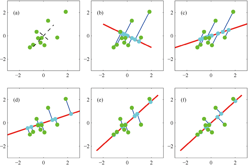
(a) A set of green data points and the true principal components (shown as eigenvectors scaled by the square root of the eigenvalues). (b) The initial configuration of the principal subspace defined by W (shown in red), and the projections of the latent points Z in the data space (given by ZWT, shown in cyan). (c) After the first M-step, W has been updated while Z is held fixed. (d) In the subsequent E-step, the values of Z have been updated and the orthogonal projections are given, and W remains fixed. (e) The result after the second M-step. (f) The converged solution.

Online EM Algorithm

An important advantage of the EM algorithm is that it can be easily implemented in Online (Online, i.e., processing data points one at a time) or Mini-batch (Mini-batch, i.e., processing a small batch of data points at a time) forms.

• Principle: In the E-step, the computations of $\mathbb{E}[\mathbf{z}_n]$ and $\mathbb{E}[\mathbf{z}_n\mathbf{z}_n^T]$ are performed separately for each data point $\mathbf{x}_n$. In the M-step, the parameter update depends on the accumulated sum ($\sum_{n=1}^N \cdots$) of the expectations over all data points.
• Implementation: We can read data points $\mathbf{x}_n$ one by one, immediately compute their $\mathbb{E}[\mathbf{z}_n]$ and $\mathbb{E}[\mathbf{z}_n\mathbf{z}_n^T]$, and then incrementally accumulate these values into the sum. After processing a data point, it can be discarded from memory.
• Advantage: The memory consumption of this method is $O(DM)$ (storing the accumulated sum), rather than $O(ND)$ (storing the entire dataset). When the amount of data $N$ is very large and cannot be loaded into memory at once, this online form is crucial.

Handling Missing Data

A powerful feature of probabilistic PCA is its ability to naturally handle Missing Data.

• It is assumed that the data is “missing at random” (MAR), i.e., the probability that a value is missing does not depend on the value itself (but can depend on other observed values).
• Method: For data points $\mathbf{x}_n$ that contain missing values, in the E-step and M-step we only compute over the observed variables. Specifically:
  • When computing the posterior distribution $p(\mathbf{z}_n | \mathbf{x}_n, \mathbf{W}, \sigma^2)$, only the observed part of $\mathbf{x}_n$ is used.
  • When updating parameters, the sum is taken only over the observed variables.
• Result: Through the EM algorithm, we can simultaneously estimate the model parameters and perform imputation of the missing values, i.e., predict the missing values based on the model and the observed data.

Nonlinear Latent Variable Models

PCA and its probabilistic version assume that the data lies in a Linear Subspace (Linear Subspace, i.e., a line, plane, or high-dimensional hyperplane). This means the data points are roughly distributed along a line, a plane, or a high-dimensional hyperplane.

However, many real-world datasets have complex, nonlinear structures. For example, an “S”-shaped curve dataset cannot be well approximated by a straight line. Linear models lose important structural information in this case.

Nonlinear Manifold

Intuition: Imagine a crumpled piece of paper — it is essentially 2D, but embedded in 3D space, and cannot be approximated by a plane. The nonlinear manifold model is meant to learn to “flatten” this crumpled data.

To capture the nonlinear structure in the data, we need to generalize the linear mapping $\mathbf{x} = \mathbf{W}\mathbf{z} + \mathbf{\mu} + \mathbf{\epsilon}$ into a Nonlinear Mapping. This is where deep neural networks come in — using a network to learn this complex nonlinear function.

• Generative process:
  1. Sample the latent variable $\mathbf{z}$ from a prior distribution (usually the standard normal distribution): $$p(\mathbf{z}) = \mathcal{N}(\mathbf{z} | \mathbf{0}, \mathbf{I})$$
  2. Map $\mathbf{z}$ to the data space through a Nonlinear Function $f(\mathbf{z}; \mathbf{w})$. This function is usually implemented by a Deep Neural Network (DNN, i.e., a neural network with multiple hidden layers, see Part 3 notes), with parameters $\mathbf{w}$.
  3. Add noise $\mathbf{\epsilon}$ (usually assumed to be Gaussian noise $\mathcal{N}(\mathbf{\epsilon} | \mathbf{0}, \sigma^2\mathbf{I})$) to get the observed data $\mathbf{x}$: $$\mathbf{x} = f(\mathbf{z}; \mathbf{w}) + \mathbf{\epsilon}$$
• Model expression: The conditional distribution of the observed data is: $$p(\mathbf{x} | \mathbf{z}, \mathbf{w}) = \mathcal{N}(\mathbf{x} | f(\mathbf{z}; \mathbf{w}), \sigma^2\mathbf{I})$$

Likelihood Function

In probabilistic models, our goal is to maximize the Marginal Likelihood or Evidence:

This integral marginalizes over all possible latent variables $\mathbf{z}$.

• Problem: In nonlinear models, since $f(\mathbf{z}; \mathbf{w})$ is a complex nonlinear function, this integral is usually intractable to compute analytically.
• Approximation method: An intuitive method is to use Monte Carlo Integration (i.e., using random sampling to approximate an integral, introduced at the beginning of this chapter) to approximate: $$p(\mathbf{x} | \mathbf{w}) \approx \frac{1}{K} \sum_{i=1}^K p(\mathbf{x} | \mathbf{z}_i, \mathbf{w}) \quad \text{where} \quad \mathbf{z}_i \sim p(\mathbf{z})$$ This approximates the marginal likelihood as a mixture of Gaussians (i.e., a weighted sum of multiple Gaussian distributions, introduced earlier in this chapter).

Why is the Monte Carlo approximation impractical in practice?

• Scenario: Consider a trained model, and we want to evaluate the likelihood of a real data point $\mathbf{x}$ (as in the figure below).
• Model generation: We sample $\mathbf{z}_i$ from the prior $p(\mathbf{z})$, and generate an image $\hat{\mathbf{x}}_i$ through $f(\mathbf{z}_i; \mathbf{w})$.
• Problem: Even if the model can generate good digits overall, the probability that a generated image $\hat{\mathbf{x}}_i$ exactly matches the real image $\mathbf{x}$ in pixel space is extremely low. For example:
  • Figure (b) is a very poor “2”, with a squared distance of 0.0387 from (a).
  • Figure (c) is a very good “2”, only shifted down and to the right by half a pixel, but its squared distance from (a) is as high as 0.2693.
• Likelihood computation: Since $p(\mathbf{x} | \mathbf{z}_i, \mathbf{w})$ is a Gaussian distribution, its value is proportional to $\exp(-\|\mathbf{x} - f(\mathbf{z}_i; \mathbf{w})\|^2 / (2\sigma^2))$.
• Dilemma:
  • If we set $\sigma^2$ very small to ensure that only very close images have high likelihood, then even a semantically perfect image like (c) will have extremely low likelihood due to tiny pixel-level shifts.
  • If we set $\sigma^2$ very large, then all images (including bad images like (b)) will have higher likelihood, losing the ability to distinguish good from bad.
• Conclusion: To get an accurate likelihood estimate, we need a huge value of $K$, so that in sampling we can occasionally generate a $\hat{\mathbf{x}}_i$ almost identical to $\mathbf{x}$. This is computationally impractical.

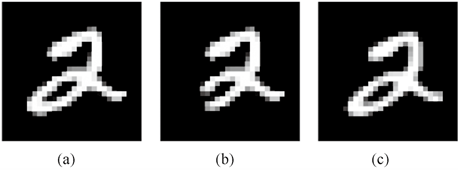
Handwritten digits, why sampling from the latent space to compute the likelihood function requires large samples

Since directly maximizing the marginal likelihood is infeasible, we need more advanced techniques to train nonlinear latent variable models. This leads to the four main methods introduced in subsequent chapters.

Discrete Data

When the observed data is discrete (such as binary or categorical variables), we need to use different conditional distributions.

• Independent binary variables: If the dataset consists of $D$ independent Binary Variables (Binary Variable, i.e., variables that take only 0 or 1), we can use a product of Bernoulli Distributions (Bernoulli Distribution, introduced in Part 2 notes):

  $$p(\mathbf{x} | \mathbf{z}, \mathbf{w}) = \prod_{i=1}^D g_i(\mathbf{z}, \mathbf{w})^{x_i} (1 - g_i(\mathbf{z}, \mathbf{w}))^{1-x_i}$$

  where $g_i(\mathbf{z}, \mathbf{w}) = \sigma(a_i(\mathbf{z}, \mathbf{w}))$ is the activation value of the i-th output unit, $\sigma(\cdot)$ is the Logistic Sigmoid Function (i.e., $\sigma(x) = 1/(1+e^{-x})$, mapping any real number to between 0 and 1, see Part 3 notes), and $a_i(\mathbf{z}, \mathbf{w})$ is the Pre-activation (Pre-activation, i.e., the linear output of the network’s last layer). This corresponds to a neural network whose output layer uses a sigmoid activation function.

• One-hot encoded categorical variables: For categorical variables, we use the multinomial distribution:

  $$p(\mathbf{x} | \mathbf{z}, \mathbf{w}) = \prod_{i=1}^D g_i(\mathbf{z}, \mathbf{w})^{x_i}$$

  where $g_i(\mathbf{z}, \mathbf{w})$ is given by the Softmax Function (Softmax Function, which converts a set of real numbers into a probability distribution whose outputs sum to 1, see Part 3 notes):

  $$g_i(\mathbf{z}, \mathbf{w}) = \frac{\exp(a_i(\mathbf{z}, \mathbf{w}))}{\sum_j \exp(a_j(\mathbf{w}))}$$

  This corresponds to a neural network whose output layer uses the softmax activation function.

• Mixed variables: For mixed data containing both discrete and continuous variables, it can be modeled by multiplying the corresponding conditional distributions.

Quantization and Dequantization

In practice, even continuous variables (such as image pixel intensities) are represented in computers by discrete values (such as 8-bit integers 0-255). This causes problems when using generative models based on deep neural networks.

• Problem: Highly flexible models may discover a “pathological” solution: collapsing the probability density entirely onto one or a few discrete values. For example, the model might always predict a pixel value of 128, resulting in very poor generated images.
• Solution: Dequantization:
  • Idea: “Dequantize” the discrete observed value into a continuous random variable.
  • Method: During training, replace each observed discrete value $x$ with a value randomly sampled from a continuous distribution. The most common is Uniform Dequantization: if $x$ is an 8-bit integer, replace it with $\tilde{x} \sim \text{Uniform}(x, x+1)$.
  • Effect: This is equivalent to adding uniform noise to the data. It makes it harder for the model to precisely collapse the density onto integer points, thereby encouraging the model to learn a smoother, more realistic distribution.

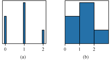
(a): A schematic of a discrete distribution. (b): The corresponding dequantized continuous distribution, a uniform distribution over the interval, whose total probability mass is the same as (a). The discrete values are "smeared" into a continuous interval.

Chapter 16 Summary

One-sentence version: Continuous latent variable models are “finding the shadow” — PCA finds the best projection direction (linear), probabilistic PCA adds a probabilistic interpretation to the projection, and nonlinear models use neural networks to learn curved projections.

Knowledge map:

1
Continuous Latent Variables
2
├── PCA (linear dimensionality reduction)
3
│   ├── Maximum variance: projection direction = direction of maximum variance
4
│   ├── Minimum error: projection direction = direction of minimum reconstruction error
5
│   ├── Data compression: represent D-dimensional data with M-dimensional projection coefficients
6
│   └── Whitening: turn the data into a standard sphere
7
├── Probabilistic PCA (probabilistic version)
8
│   ├── Generative model: z -> Wz + noise -> x
9
│   ├── Maximum likelihood: the solution for W is consistent with PCA
10
│   └── EM algorithm: E-step guesses z, M-step updates W
11
├── Other models
12
│   ├── Factor Analysis: different noise per dimension
13
│   ├── ICA: independent non-Gaussian latent variables
14
│   └── Kalman Filter: sequential latent variables
15
├── ELBO: lower bound of the log-likelihood
16
└── Nonlinear manifold: use neural networks to learn curved projections

These methods play an important role in data compression, feature extraction, and visualization.

Thanks for reading! Follow me if you'd like~

Deep Learning Notes - 7: Sampling Methods and Latent Variable Models

Mon Sep 01 2025

9267 words · 49 minutes

NotesDeep LearningLearningSamplingLatent VariablePCAEM Algorithm

---

© MuxiaoWF | CC BY-NC-SA 4.0

Share

Share this article

X (Twitter)TelegramRedditFacebookEmailQQ

Close

Close