Part 6/8 of the series ← Previous | Next | Glossary

It is recommended to read Parts 1-5 first, especially Part 5 on CNNs (to understand the convolution→attention evolution) and Part 4 on residual connections. This part covers the Transformer attention mechanism, why it is stronger than RNNs, and how graph neural networks handle non-grid data.

Chapter 12 Transformer

Attention

Attention is the core concept of the Transformer model. It allows a neural network, when processing sequential data, to dynamically assign different importance weights to different inputs. These weights themselves also depend on the input data, enabling the model to capture dependencies within the sequence.

Unlike the fixed weights in traditional neural networks, the weights of the attention mechanism are data-dependent, i.e., they are computed dynamically based on the current input.

Consider the following two sentences:

1. I swam across the river to get to the other bank.
2. I walked across the road to get cash from the bank.

The same word “bank” has different meanings in different contexts (river bank vs. bank/financial institution). The model needs to determine its correct meaning based on the other words in the context (such as “swam”, “river”, “cash”).

This shows that when processing a word, the model should “attend to” other words in the sequence that are relevant to it. The degree of attention (weight) depends on the input sequence itself.

• Traditional word embeddings: each word is mapped to a fixed vector (e.g., “bank” is always the same vector), and cannot distinguish polysemous words.
• The goal of the Transformer: through the attention mechanism, map words into a new representation space, so that the same word obtains different vector representations in different contexts.
  • In the first sentence, the representation of “bank” will be close to “water”.
  • In the second sentence, the representation of “bank” will be close to “money”.

The input to the Transformer is a set of vectors $\{x_n\}$, where $n = 1, \dots, N$.

• Each vector $x_n$ is called a token.
  • In NLP, a token can be a word, a subword, or a character.
  • In images, a token can be an image patch.
  • In protein sequences, a token can be an amino acid.
• Each element of the vector $x_n$ is called a feature.
• The vector dimension is $D$, and the sequence length is $N$.

We organize the inputs into an $N \times D$ matrix $X$:

Therefore the basic unit of a Transformer is a function that transforms the input matrix $X$ into an output matrix $\tilde{X}$, keeping the dimension unchanged:

Multiple such layers can be stacked to form a deep network. Each layer has its own learnable parameters (weights and biases), trained via gradient descent.

A Transformer layer consists of two main stages:

1. Attention mechanism: mix information from different tokens along the column direction (feature dimension).
2. Per-row transformation: perform feature transformation within each row (each token).

Attention Coefficients

Imagine that while reading an article, in order to understand a certain sentence, you need to “attend to” certain parts of the article. The attention mechanism is what enables machine learning to do the same.

Goal: map the input vectors $x_1, \dots, x_N$ to output vectors $y_1, \dots, y_N$, so that the representation of $y_n$ is richer.

Key idea: the output vector $y_n$ depends not only on the corresponding input $x_n$ (a single input vector), but also on all the other inputs $x_1, \dots, x_N$ (the overall meaning). The degree of dependence is controlled by the attention weight $a_{nm}$.

Define each output vector as a linear combination of the input vectors:

The attention weights $a_{nm}$ should satisfy:

1. Non-negativity: $a_{nm} > 0$ (to avoid positive-negative cancellation)
2. Normalization: $\sum_{m=1}^{N} a_{nm} = 1$ (to ensure the weights sum to 1)

These two constraints mean that $a_{nm} \in [0, 1]$, i.e., the weights form a “partition of unity”.

• If $a_{nn} = 1$ and $a_{nm} = 0$ (when $m \neq n$), then $y_n = x_n$, and the input is unchanged.
• In general, $y_n$ is a weighted average of all input vectors, with the weights determined by the input data.

In summary, the attention mechanism enables the model to focus on important parts of the input sequence by dynamically allocating weights.

Suppose we have 3 input vectors:

• $x_1 = [1, 2, 3]$ (e.g., describing a “cat”)
• $x_2 = [4, 5, 6]$ (e.g., describing a “dog”)
• $x_3 = [7, 8, 9]$ (e.g., describing an “animal”)

We want to compute the output vector $y_1$: $y_1 = a_{11} \times x_1 + a_{12} \times x_2 + a_{13} \times x_3$

Suppose the attention coefficients are:

• $a_{11} = 0.5$ (50% attention to itself)
• $a_{12} = 0.3$ (30% attention to the second input)
• $a_{13} = 0.2$ (20% attention to the third input)

Then:

The focus can also be adjusted dynamically:

• $y_1$ may focus more on the “cat” information ($a_{11}=0.7, a_{12}=0.2, a_{13}=0.1$)
• $y_2$ may focus more on the “dog” information ($a_{21}=0.2, a_{22}=0.7, a_{23}=0.1$)
• $y_3$ may focus more on the overall concept ($a_{31}=0.3, a_{32}=0.3, a_{33}=0.4$)

Self-Attention

How are the attention weights $a_{nm}$ computed?

First, through an information retrieval analogy:

• Key: describes the attributes of an item (e.g., a movie’s genre, actors).
• Value: the item itself (e.g., the movie file).
• Query: the user’s preference (e.g., the genre they want to watch).

The system finds the best match by comparing the Query and the Key, and returns the corresponding Value.

In the Transformer, however:

• Value: the input vector $x_n$ is used directly as the Value.
• Key: the input vector $x_n$ is also used as the Key.
• Query: the input vector $x_m$ is used as the Query for the output $y_m$.

This is called “self-attention” because the Query, Key, and Value all come from the same input sequence.

To compute the similarity between Query $x_n$ and Key $x_m$. A simple method is the dot product; a larger dot product indicates that the two words are more related:

Use the Softmax function to convert the dot product into normalized attention weights:

Softmax ensures the non-negativity and normalization of the weights.

Organize all attention weights into an $N \times N$ matrix:

where $\text{Softmax}(L)$ means taking the exponential of each element of the matrix $L$, and then normalizing each row.

The output matrix $Y$ is:

Suppose the input sequence has 3 words:

Compute the similarity matrix:

Apply Softmax to each row to get the attention weights:

Finally compute the final output Y.

Network Parameters

The above self-attention mechanism has no learnable parameters, so it cannot learn from data. Moreover, all features have the same weight when computing similarity.

Solution: apply a linear transformation to the inputs, introducing learnable weight matrices.

Definitions:

• Query matrix: $Q = X W^{(q)}$
• Key matrix: $K = X W^{(k)}$
• Value matrix: $V = X W^{(v)}$

where $W^{(q)}, W^{(k)}, W^{(v)}$ are learnable weight matrices.

Dimension notes:

• $W^{(k)}$ and $W^{(q)}$ have dimensions $D \times D_k$, ensuring that $Q$ and $K$ have the same number of columns so that the dot product $Q K^T$ can be computed.
• $W^{(v)}$ has dimensions $D \times D_v$, determining the dimension of the output vector.
• Usually set $D_k = D$, $D_v = D$ to keep the input and output dimensions consistent, which facilitates stacking layers and using residual connections.

The final self-attention output is:

Scaled Self-Attention

Problem: when $D_k$ is large, the variance of the dot product $q_n^T k_m$ becomes very large (about $D_k$), causing the input to the Softmax function to become too large, pushing it into the saturated region where the gradient is very small, which harms training.

Solution: scale the dot product result by dividing by $\sqrt{D_k}$.

The final self-attention formula is:

Multi-Head Attention

A single attention head may only capture one type of dependency (such as syntactic or semantic relations).

Solution: use multiple parallel attention heads, each learning a different projection space, thereby capturing different types of patterns.

Define $H$ heads:

• The output of the $h$-th head is: $H_h = \text{Attention}(Q_h, K_h, V_h)$
• where: $$Q_h = X W_h^{(q)}, \quad K_h = X W_h^{(k)}, \quad V_h = X W_h^{(v)}$$
• Each head has its own independent learnable parameters $W_h^{(q)}, W_h^{(k)}, W_h^{(v)}$.

Concatenate the outputs of all heads:

The dimension is $N \times (H \cdot D_v)$.

Then project back to the original dimension $D$ via a linear transformation $W^{(o)}$:

where $W^{(o)}$ has dimensions $(H \cdot D_v) \times D$.

Usually set $D_v = D / H$, so that the concatenated dimension is exactly $N \times D$.

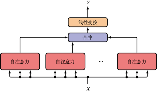
Information flow of multi-head attention

Transformer Layer

Multi-head self-attention is the core of the Transformer. To build a deep network, multiple layers need to be stacked.

To improve training, residual connections (see Chapter 9 - Residual Connections) and Layer Normalization (Layer Normalization, which independently normalizes the feature vector of each token to stabilize training) are introduced:

Let the output of multi-head attention be $Y(X)$, then the result after adding the residual connection and layer normalization is:

This ensures that even if the attention layer learns nothing ($Y(X) \approx 0$), information can still pass through the residual path $X$.

“Pre-normalization” can also be used:

The output of the attention layer is a linear combination of the input vectors (via the attention weights), which limits its expressiveness.

To introduce nonlinear transformations, a Multi-Layer Perceptron (MLP) is usually added after the attention layer:

• For example, a two-layer fully connected network, using the ReLU activation function in between.
• Residual connections and layer normalization are also used.

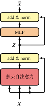
A complete Transformer layer: the input $X$ goes through multi-head self-attention (with residual and normalization) to get $Z$, then $Z$ goes through the MLP (a multi-layer network, with residual and normalization) to get the final output $\tilde{X}$, containing two sub-layers:

1. Multi-head self-attention sub-layer (highlighting relations)

• Receives input $X$.
• Computes the multi-head attention output $Y(X)$.
• Applies the residual connection: $X + Y(X)$. (stabilizes representation)
• Applies layer normalization: $Z = \text{LayerNorm}(X + Y(X))$.

• Input X → multi-head self-attention → Y(X) → residual connection + layer normalization → Z

2. Feed-forward neural network sub-layer (enriching representation)

• Receives the output $Z$ from the previous step.
• Performs a nonlinear transformation via a fully connected MLP. The usual structure is: $$\text{MLP}(z) = W_2 \cdot \text{ReLU}(W_1 \cdot z + b_1) + b_2$$ where $W_1$ typically has dimensions $D \times D_{ff}$ ($D_{ff} > D$, e.g., 4 times), and $W_2$ has dimensions $D_{ff} \times D$, ensuring the output dimension matches the input.
• Applies the residual connection: $Z + \text{MLP}(Z)$.
• Applies layer normalization: $\tilde{X} = \text{LayerNorm}(Z + \text{MLP}(Z))$.

• Z → MLP → MLP(Z) → residual connection + layer normalization → final output X̃

The final output $\tilde{X}$ has the same dimension as the input $X$, which is $N \times D$.

By stacking multiple such Transformer layers, a deep network can be built:

where $X^{(0)}$ is the initial input (usually word embeddings plus positional encoding), and $X^{(L)}$ is the final representation, which can be used for downstream tasks (such as classification, generation, etc.).

Positional Encoding

The self-attention mechanism has a key property: it is permutation invariant or order-independent.

From the formula $Y = \text{Softmax}(QK^T / \sqrt{D_k}) V$, it can be seen that the computation depends only on the dot products and linear combinations between vectors. If we arbitrarily reorder the rows of the input sequence $X$ (i.e., the tokens), as long as we apply the same permutation to $Q, K, V$, the final output $Y$ will be the result of the same permutation.

However, in most sequence tasks (especially NLP), order is crucial. For example, “the cat chases the mouse” and “the mouse chases the cat” have completely different meanings. A standard self-attention layer cannot distinguish between these two cases.

To enable the model to exploit sequence order, positional information (the index $n$ of a token in the sequence) must be explicitly injected into the input. (Add a “position label” to the words)

The most common method is positional encoding: Add the positional encoding vector $p_n$ to the input embedding vector $x_n$ of the $n$-th token:

In matrix form, add the positional encoding matrix $P$ to the input matrix $X$:

where $P$ is an $N \times D$ matrix, and the $n$-th row is the encoding vector $p_n$ for position $n$.

The positional encoding vector $p_n$ must satisfy:

1. Uniqueness: each position $n$ has a unique encoding.
2. Learnable or deterministic: the encoding can be a learnable parameter or a predefined function.

Sine/cosine encoding:

Use sine and cosine functions of different frequencies to generate $p_n$. For position $n$ and dimension $i$:

where $i = 0, 1, \dots, D/2 - 1$.

Characteristics:

• Deterministic: the encoding is precomputed and not learnable.
• Periodicity: different dimensions have different wavelengths (controlled by $L$).
• Relative position: the model can relatively easily learn the relationship between $p_{n+k}$ and $p_n$ (e.g., via a linear transformation), which helps capture relative positional information.

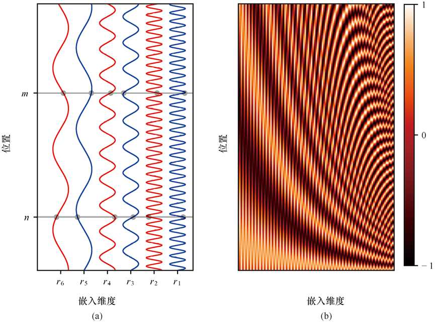
(a) In the figure, the horizontal axis represents the different components of the embedding vector r_n, and the vertical axis represents the position in the sequence. The vector element values at position n and position m are both given by the intersections of the corresponding sine and cosine curves with the horizontal gray lines. (b) Heat map of the positional encoding vectors defined by the above equation for the first N=200 positions with L=30, where the dimension is D=100

Learnable positional encoding

A simpler method is to treat the positional encoding $P$ as a learnable parameter. Initialize an $N_{\text{max}} \times D$ matrix ($N_{\text{max}}$ is the maximum sequence length supported by the model), where each row corresponds to the encoding vector of a position. During training, these vectors are optimized together as model parameters.

This method usually performs well in practice and is simple to implement.

When $x_n$ becomes $x_n + p_n$, when computing the Query, Key, and Value:

The positional information $p_n$ is encoded into $q_n, k_n, v_n$. Therefore, when computing the attention weights $\text{Softmax}(QK^T / \sqrt{D_k})$, the dot product $q_n^T k_m$ depends not only on the semantics of $x_n$ and $x_m$, but also on their positions $n$ and $m$. This enables the model to distinguish sequences with different orders.

Each token of the input sequence is added a position-dependent vector, and then this augmented sequence representation is fed into the first Transformer layer.

Natural Language

Natural language (such as English, Chinese) is essentially a sequence of symbols. A sentence can be viewed as an ordered list composed of words and punctuation marks, which are usually separated by spaces. For example: ["The", "cat", "sat", "on", "the", "mat", "."]

This sequentiality is the core of language understanding. Changing the word order usually changes the meaning of the sentence, or even makes it meaningless. For example:

• "The cat chased the dog." (the cat chases the dog)
• "The dog chased the cat." (the dog chases the cat)
• "Chased cat the dog the." (grammatically incorrect, hard to understand)

Therefore, models that process language must be able to capture and exploit long-range dependencies in the sequence, such as the dependency between the subject and the verb, even when they are far apart.

one-hot encoding: One-hot encoding maps each word to a vector of length equal to the vocabulary size, where only one element is 1 and the rest are 0. For example, for a vocabulary of size 10, the one-hot encoding of the word “cat” is: [0, 0, 1, 0, 0, 0, 0, 0, 0, 0]. Each word occupies an independent dimension in the vocabulary.

Word Embeddings

One-hot encoding suffers from high dimensionality (when the vocabulary is large) and the inability to capture relationships between words. Word embeddings solve these problems by mapping words to low-dimensional dense vectors.

• Embedding matrix definition: Let the embedding space dimension be D and the vocabulary size be K, then the embedding matrix E has dimensions $D \times K$. For a one-hot encoded input vector $x_n$, its corresponding embedding vector is: $$v_n = E x_n$$ Since $x_n$ is a one-hot vector, $v_n$ is essentially the corresponding column vector of the matrix E.
• Word2vec model:
  • A method that learns word embeddings through a two-layer neural network, based on self-supervised learning (generating training samples from unlabeled text).
  • Two variants:
    • Continuous Bag of Words (CBOW): uses the context words in a window as input to predict the center word (a “fill-in-the-blank” task).
    • Skip-gram: uses the center word as input to predict the context words in the window.

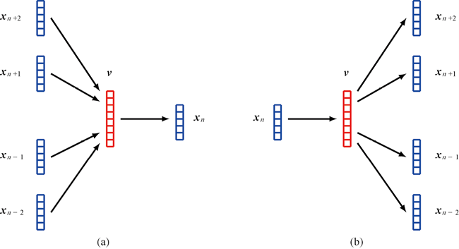
      Word2vec model: left is the bag-of-words model, right is the skip-gram model

• Semantic properties of word embeddings:
  • Semantically related words are closer in the embedding space (e.g., “Paris” and “London”).
  • Supports simple vector arithmetic, for example: $v(\text{Paris}) - v(\text{France}) + v(\text{Italy}) \simeq v(\text{Rome})$
• Application methods:
  • As a pretrained layer, the pretrained embedding matrix can be fixed, or used as a learnable layer in end-to-end training (the initial values can be random or use the pretrained matrix).

Tokenization

A fixed vocabulary cannot handle out-of-vocabulary words or spelling errors, while character-level processing loses word structure and is computationally expensive.

• Goal: combine the advantages of word-level and character-level processing, converting text into tokens (groups of characters, which may contain complete words, word fragments, or single characters).
• Byte Pair Encoding (BPE):
  • Process: starting from individual characters, iteratively merge the most frequent adjacent token pairs (without merging across words), until a preset number of tokens is reached.
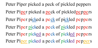
  • As shown in the figure, first merge “pe” (appears 4 times, excluding “Pe""), then merge “ck” (appears 3 times), and so on.
• Advantages: handles out-of-vocabulary words, preserves word structure, and supports multimodal (e.g., code) processing.

Bag of Words Model

• Joint distribution assumption: assume that words in the sequence are independent, and the joint distribution decomposes as: $$p(x_1, ..., x_N) = \prod_{n=1}^N p(x_n)$$ completely ignoring word order (hence the name “bag of words”).
• Text classification application:
  • Naive Bayes classifier: assumes words are independent within each class, and the class-conditional probability is: $$p(x_1, ..., x_N | \mathcal{C}_k) = \prod_{n=1}^N p(x_n | \mathcal{C}_k)$$
  • Posterior probability computation: $$p(\mathcal{C}_k | x_1, ..., x_N) \propto p(\mathcal{C}_k) \prod_{n=1}^N p(x_n | \mathcal{C}_k)$$
• Smoothing: when a word appears in the test set but not in training, its probability would be 0; smoothing (e.g., uniformly assigning small probabilities) is needed to avoid this.

Autoregressive Models

• Joint distribution decomposition: considering word order, decompose the joint distribution into a product of conditional probabilities: $$p(x_1, ..., x_N) = \prod_{n=1}^N p(x_n | x_1, ..., x_{n-1})$$
• n-gram model:
  • Simplified assumption: the conditional probability depends only on the previous L words (e.g., L=1 is bigram, L=2 is trigram).
  • Example (L=2): $$p(x_1, ..., x_N) = p(x_1) p(x_2 | x_1) \prod_{n=3}^N p(x_n | x_{n-1}, x_{n-2})$$
• Limitations:
  • Parameter explosion: as L grows, the size of the probability table grows exponentially (difficult to exceed trigram).
  • Long-range dependencies: cannot capture long-distance inter-word relations, and the generated text may be incoherent.
• Hidden Markov Model (HMM): passes long-range information through latent variables, but has limited capacity (depends on the latent state chain).

Recurrent Neural Networks (RNN)

• Motivation: solve the problems of variable sequence length and parameter sharing, supporting equivariance (the same word has consistent semantics at different positions).
• Structure:
  • Introduce a hidden state $z_n$; the input is the current word $x_n$ and the previous hidden state $z_{n-1}$, and the output is the current word $y_n$ and the new hidden state $z_n$.
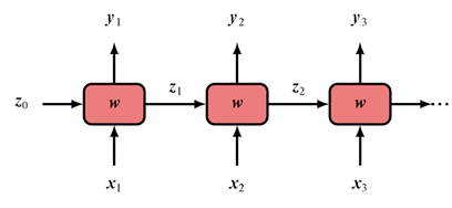
  • Weights are shared across sequence positions, as shown in the figure (the initial hidden state $z_0$ is usually set to an all-zero vector).
• Machine translation example:
  • Encoder: processes the input sequence (e.g., English) and compresses it into a hidden state $z^*$.
  • Decoder: starting from $z^*$ and the $\langle \text{start} \rangle$ token, generates the output sequence (e.g., Dutch) until the $\langle \text{end} \rangle$ token, as shown in the figure below.
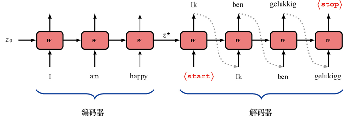
  • Autoregressive property: each output word is used as the next input, similar to the autoregressive formula above.

Backpropagation Through Time

• Training method: compute gradients via backpropagation, with the error function being cross-entropy (the output uses softmax activation).
• Problems:
  • Vanishing/exploding gradients: during training on long sequences, gradients decay or explode after passing through many steps.
  • Poor long-range dependency: the input sequence must be compressed into a fixed-length $z^*$, and long sequences easily lose information (bottleneck problem).
• Improved models:
  • LSTM (Long Short-Term Memory) and GRU (Gated Recurrent Unit): enhance long-range information retention through gating mechanisms.
• Limitations:
  • Poor parallel computation: sequence processing depends on previous steps, and cannot efficiently utilize GPUs.
  • Still limited by the ability to model long-range dependencies.

Transformer Language Models

Divided into three categories by input-output form:

• Encoder model: input a sequence, output a fixed vector (e.g., sentiment analysis).
• Decoder model: input a vector, output a sequence (e.g., text generation).
• Sequence-to-sequence model: both input and output are sequences (e.g., translation).

Decoder Transformer

• GPT model: Generative Pretrained Transformer, an autoregressive model whose goal is to learn the conditional probability $p(x_n | x_1, ..., x_{n-1})$.
• Architecture:
  • Input: token sequence $x_1, ..., x_N$ (including positional encoding).
  • Output: obtain the token probability distribution via linear transformation + softmax: $$Y = \text{Softmax}(\tilde{X} W^{(p)})$$
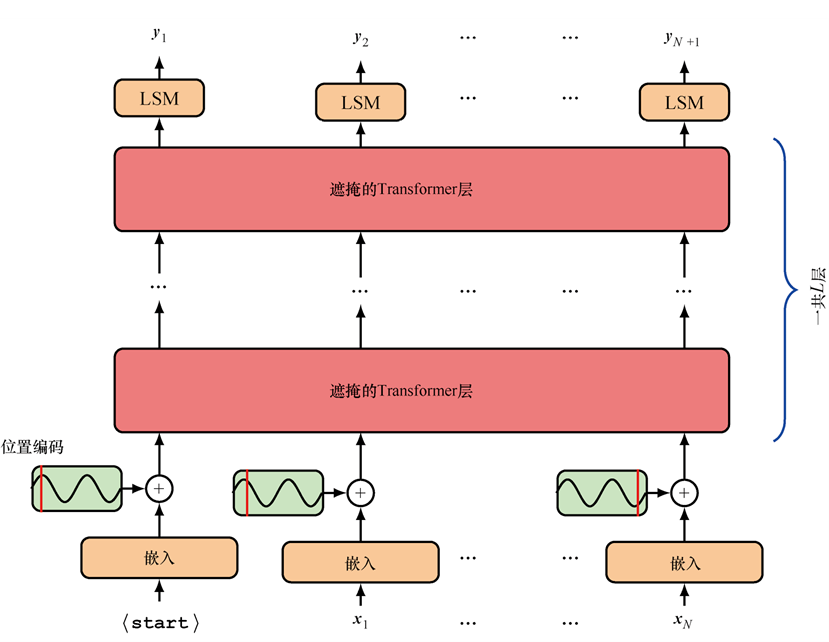
• Training method:
  • Self-supervised learning: take a sequence from unlabeled text and train with $x_{n+1}$ as the target.
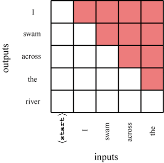
  • Parallel processing: split the sequence into multiple subsequences (e.g., “I swam across the river” is split into “I swam” → “across”, “I swam across” → “the river”, etc.).
  • Masked attention (causal attention): ensure that when predicting $x_n$, only previous tokens are attended to, as shown in the figure below (attention weights in the red region are set to 0).
• Sequence processing:
  • Padding token $\langle \text{pad} \rangle$: unifies sequences of different lengths, and the attention of $\langle \text{pad} \rangle$ is ignored via masking.
  • Generation process: each time sample the next token and add it to the sequence, looping until the $\langle \text{end} \rangle$ token.

Sampling Strategies

• Greedy search: each time select the token with the highest probability; deterministic but may not be the optimal sequence.
• Beam search:
  • Keep the B best hypotheses (beam width B), each time expand to $B^2$, then filter out B.
  • Needs length normalization (to avoid bias toward short sequences); computational cost is $O(BKN)$.
• Random sampling:
  • Top-K sampling: sample from the K tokens with the highest probability according to normalized probabilities.
  • Top-p sampling (nucleus sampling): sample from the set of tokens whose cumulative probability reaches the threshold p.
  • Temperature parameter: adjusts the softmax distribution: $$y_i = \frac{\exp(a_i / T)}{\sum_j \exp(a_j / T)}$$ $T \to 0$ approaches greedy, T=1 is the original distribution, $T \to \infty$ tends toward uniform.
• Problems: greedy/beam search may repeat sequences, random sampling may generate meaningless text (human text has lower probability but is more reasonable).

Encoder Transformer

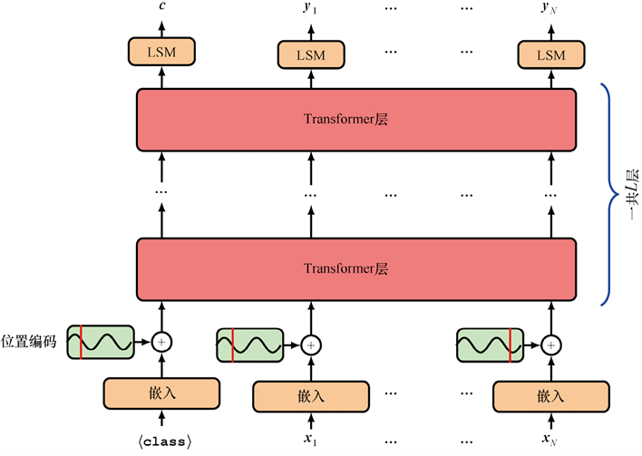
• BERT model: Bidirectional Encoder Representations, pretrained and then fine-tuned to adapt to downstream tasks.
• Pretraining method:
  • Randomly select 15% of tokens to replace with $\langle \text{mask} \rangle$ (80%), a random word (10%), or keep the original word (10%), training the model to predict the original word.
  • Bidirectionality: allows attending to both preceding and following tokens, without needing to shift the input right or use masking, as shown in the structure below.
• Fine-tuning:
  • Classification tasks: use the output of the first $token$, followed by a linear layer + softmax.
  • Token-level tasks: use all outputs, followed by a shared linear layer + softmax.
• Limitation: low training efficiency (only some tokens are targets), and cannot generate sequences.

Sequence-to-Sequence Transformer

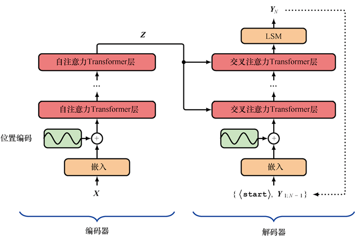
• Application: e.g., translation (input English, output Dutch), combining an encoder and a decoder.
• Cross-attention: the decoder’s Query $Q$ comes from the generated sequence, and the Key $K$ and Value $V$ come from the encoder’s output $Z$.
• Overall architecture: as shown in the figure below, the encoder processes the input sequence, and the decoder combines the encoder’s output through cross-attention to generate the target sequence.

Large Language Models (LLMs)

• Scale: parameters reach the trillion level (e.g., GPT-4), relying on large-scale text data and parallel computation (GPU clusters).
• Training paradigm:
  • Self-supervised pretraining: learn language patterns on massive unlabeled text.
  • Fine-tuning: adapt to downstream tasks via a small amount of labeled data (transfer learning).
• Low-Rank Adaptation (LoRA):
  • Freeze the pretrained model weights, add low-rank matrices ($A (D \times R)$) and ($B (R \times D)$), and the output is ($X W_0 + XAB$).
  • After fine-tuning, merge weights: $\hat{W} = W_0 + AB$, reducing the number of parameters (e.g., by 1/10000).
• Prompt engineering: guide the model to complete tasks by designing input prompts (e.g., “translate: …”), supporting few-shot learning.
• RLHF: optimize model outputs via Reinforcement Learning from Human Feedback (e.g., ChatGPT).

Multimodal Transformer

• Core: convert different modalities (text, image, audio, etc.) into tokens, and process them uniformly with a Transformer.

Vision Transformer

• Image tokenization:
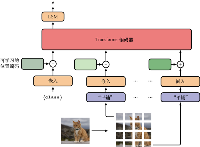
  • Split the image $H \times W \times C$ into $P \times P$ non-overlapping patches (e.g., $P=16$), and flatten them into vectors.
  • Or use a small CNN for downsampling to generate tokens.
• Architecture: as shown in the figure below, add a $token$ and learnable positional encoding, and output the classification result through the encoder.
• Characteristics: weak inductive bias (relies on data to learn image geometric properties), requires more training data, but may achieve higher accuracy.

Generative Image Transformer

• Autoregressive generation: predict pixels in raster scan order (reading order), with the joint distribution decomposed as: $p(x_1, ..., x_N) = \prod_{n=1}^N p(x_n | x_1, ..., x_{n-1})$
• Discrete representation:
  • Vector Quantization (VQ): approximate pixel patches with a codebook $\mathcal{C}$, $x_n \to \arg\min_{c_k \in \mathcal{C}} \|x_n - c_k\|^2$, solving the blurriness problem of continuous-value generation.
  • ImageGPT: maps pixels to a discrete color codebook and uses a Transformer to learn next-token prediction.

Audio Data Processing

• Mel Spectrogram: convert the audio waveform into a time-frequency matrix (perceptually uniform frequency division).
• Audio classification:
  • Split the mel spectrogram into patches, generate tokens, and feed them into the Transformer encoder.
  • Use the $token$ output for classification results, outperforming CNNs (which excel at long-range dependencies).

Text-to-Speech

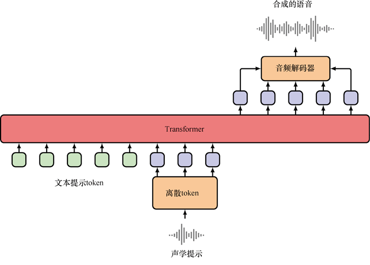
Vall-E

• Vall-E model:
  • Speech tokenization: convert speech into discrete tokens using vector quantization.
  • Input: text tokens + a few speech tokens of the target speaker, output the corresponding speech tokens, as shown in the figure above.
  • Advantage: can imitate a new speaker’s voice with only a few seconds of samples.

Vision and Language Transformer

• Data: e.g., LAION400M (text-image pairs), supporting text-to-image generation, image-to-text generation, etc.
• Parti model: encoder-decoder architecture, input text tokens, output image tokens (vector-quantized patches).
• CM3Leon model:
  • Training data: HTML documents containing text and images.
  • Supports multi-tasks such as text-image generation, image editing, and caption generation.

Chapter 12 Summary

One-sentence version:

• Attention mechanism: lets the model dynamically decide “where to look”, understood through the information retrieval analogy of Q/K/V — the better the query matches the key, the greater the weight of the corresponding value
• Self-attention: Q, K, and V all come from the same sequence, solving the disambiguation problem of whether “bank” means a river bank or a financial institution
• Multi-head attention: multiple attention heads run in parallel, each capturing a different type of dependency (syntax, semantics, etc.), then concatenate and project
• Positional encoding: add position labels to tokens, solving the “permutation invariant” shortcoming of self-attention — without it, “the cat chases the dog” and “the dog chases the cat” cannot be distinguished
• Transformer layer: attention sub-layer (mixing inter-token relations) + feed-forward sub-layer (enriching each token’s representation), stabilized by residual connections and layer normalization
• Three major architectures: encoder (BERT, bidirectional understanding), decoder (GPT, autoregressive generation), Seq2Seq (translation, etc., connected by cross-attention)

Knowledge map:

1
Self-attention (Q/K/V + Softmax)
2
    ↓ introduce learnable parameters
3
Scaled self-attention (÷√D_k to prevent saturation)
4
    ↓ parallel multiple groups
5
Multi-head attention → concatenate + linear projection
6
    ↓ add residual connection + layer normalization + feed-forward MLP
7
Transformer layer → stack L layers → deep network
8
    ↓ add positional encoding (sine/learnable)
9
    ├── Encoder (BERT): bidirectional, masked language model
10
    ├── Decoder (GPT): autoregressive, causal attention
11
    └── Seq2Seq: encoder + decoder + cross-attention

Chapter 13 Graph Neural Networks

Sequences (1D) and images (2D grids) are special cases of structured data, while more general structured data can be described by a Graph — composed of nodes and edges, where both nodes and edges can be associated with data (e.g., atom types in a molecule, travel time in a railway network).

Graph-Based Machine Learning

• Node prediction: predict node attributes (e.g., classify document topics based on hyperlinks between web pages).
• Edge prediction (graph completion): predict whether an edge exists (e.g., completing unobserved interactions in a protein-protein interaction network).
• Graph prediction (regression/classification): predict properties of an entire graph (e.g., the water solubility of a molecule), where the training data is a set of multiple independent graphs.
• Inductive learning and transductive learning:
  • Inductive learning: training and test graphs/nodes are independent (e.g., predicting the properties of a new molecule).
  • Transductive learning: the entire graph structure is known, but only some nodes are labeled, and the labels of the remaining nodes are predicted (e.g., distinguishing real humans from bots in a social network).
• Graph representation learning: learn an effective internal representation of the graph for downstream tasks (e.g., pretrain a molecule foundation model, then fine-tune it for specific tasks).

Basic Concepts and Notation of Graphs

• Definition of a graph: a graph $G=(V, E)$, where $V$ is the node set and $E$ is the edge set. Node indices $n=1,...,N$, an edge $(n,m)$ connects node $n$ and node $m$, and the neighbor set of node $n$ is denoted $\mathcal{N}(n)$.
• Node data: the attributes of each node $n$ are represented by a $D$-dimensional vector $x_n$, and all node data form an $N \times D$ matrix $X$ (row $n$ is $x_n^T$).

Adjacency Matrix

An $N \times N$ matrix $A$, where $A_{nm}=1$ if there is an edge between node $n$ and $m$, otherwise 0. For an undirected graph, $A$ is symmetric with $A_{nm}=A_{mn}$.

• Problem: the adjacency matrix depends on the node ordering, whereas the properties of a graph should be independent of the node ordering.

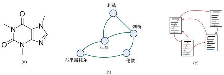
Adjacency matrix depends on node ordering

Permutation Invariance and Equivariance

• Permutation matrix: $P$ is an $N \times N$ matrix with only one 1 in each row and each column, used to represent node reordering. If node $n$ is reordered to $m=\pi(n)$, then row $n$ of $P$ is the unit vector $u_{\pi(n)}^T$.
• Data permutation:
  • Node data matrix: $\tilde{X} = PX$ with rows reordered along with the nodes.
  • Adjacency matrix: $\tilde{A} = PAP^T$ (both rows and columns are reordered).
• Network output requirements:
  • Graph-level prediction requires permutation invariance: $y(\tilde{X},\tilde{A}) = y(X,A)$.
  • Node-level prediction requires permutation equivariance: $y(\tilde{X},\tilde{A}) = Py(X,A)$ (the prediction is reordered synchronously with the nodes).

Neural Message Passing

• Goal: build a network that satisfies permutation equivariance/invariance, supports multi-layer nonlinear transformations, handles variable-length graphs, and is scalable.
• Convolutional Neural Networks (CNN, see Part 5) — an image can be viewed as a special graph (pixels as nodes, adjacent pixels as edges); CNNs aggregate information through local filters, and graph neural networks similarly aggregate information through neighbors.

Graph Convolution and the Message Passing Framework

• From CNN to graph convolution:

  • $3 \times 3$ filter in CNN: $z_i^{(l+1)} = f\left( \sum_j w_j z_j^{(l)} + b \right)$ (j is a local pixel).
  • Graph convolution modification: aggregate neighbor information, with shared parameters to ensure equivariance: $$z_i^{(l+1)} = f\left( w_{\text{neigh}} \sum_{j \in \mathcal{N}(i)} z_j^{(l)} + w_{\text{self}} z_i^{(l)} + b \right)$$ where $w_{\text{neigh}}$ (neighbor weight) and $w_{\text{self}}$ (self weight) are shared across all nodes.

• Message Passing Neural Network:

  • Process: each layer is divided into two steps, Aggregate and Update.
  • Aggregate: for node n, aggregate the neighbor embeddings: $$z_n^{(l)} = \text{Aggregate}\left( \{ h_m^{(l)} : m \in \mathcal{N}(n) \} \right)$$
  • Update: combine its own embedding with the aggregation result: $$h_n^{(l+1)} = \text{Update}\left( h_n^{(l)}, z_n^{(l)} \right)$$
  • Initialization: $h_n^{(0)} = x_n$ (the initial node embedding is its attributes).

Message Passing

Aggregation Operators

Must satisfy: independent of neighbor order, support a variable number of neighbors, and be differentiable. Common forms:

• Sum: collect information from all neighbor nodes $$\text{Aggregate}(...) = \sum_{m \in \mathcal{N}(n)} h_m^{(l)}$$ Advantage: preserves neighbor count information; disadvantage: nodes with many neighbors have excessively strong influence.
• Mean: $$\text{Aggregate}(...) = \frac{1}{|\mathcal{N}(n)|} \sum_{m \in \mathcal{N}(n)} h_m^{(l)}$$ Advantage: normalized; disadvantage: loses neighbor count information.
• Symmetric normalization: $$\text{Aggregate}(...) = \sum_{m \in \mathcal{N}(n)} \frac{h_m^{(l)}}{\sqrt{|\mathcal{N}(n)| \cdot |\mathcal{N}(m)|}}$$ balances the neighbor count differences between different nodes.
• Element-wise max/min: take the element-wise max/min of neighbor embeddings, which also satisfies permutation invariance.
• Parametric aggregation: introduce learnable parameters via an MLP (universal approximator): $$\text{Aggregate}(...) = \text{MLP}_\theta\left( \sum_{m \in \mathcal{N}(n)} \text{MLP}_\phi(h_m^{(l)}) \right)$$ where $\text{MLP}_\phi$ (neighbor transformation) and $\text{MLP}_\theta$ (post-aggregation transformation) are shared networks.

Update Operators

The new state of a node = process (aggregated information + the node’s original information)

• Basic form: combine its own embedding with the aggregation result, and update via a nonlinear transformation: $$\text{Update}(h_n^{(l)}, z_n^{(l)}) = f\left( W_{\text{self}} h_n^{(l)} + W_{\text{neigh}} z_n^{(l)} + b \right)$$ where $f$ is an activation function (e.g., ReLU), and $W_{\text{self}}, W_{\text{neigh}}$ are weight matrices.
• Simplified form: if $W_{\text{self}} = W_{\text{neigh}}$ and aggregation uses sum, then: $$h_n^{(l+1)} = f\left( W_{\text{neigh}} \sum_{m \in \mathcal{N}(n) \cup \{n\}} h_m^{(l)} + b \right)$$

Suppose we have a 3x3 image patch

• CNN: the center pixel 5 will consider the surrounding 1,2,3,4,6,7,8,9
• GNN: the center node 5 only considers directly connected nodes 1,2,6,7

Node/Edge/Graph Classification Implementation

• Node classification: (predict the class of each node in the graph)

  • Output layer: apply softmax to the final embedding $h_n^{(L)}$: $$y_{ni} = \frac{\exp(w_i^T h_n^{(L)})}{\sum_j \exp(w_j^T h_n^{(L)})}$$
  • Loss function: cross-entropy loss (only training nodes $\mathcal{V}_{\text{train}}$ participate): $$\mathcal{L} = -\sum_{n \in \mathcal{V}_{\text{train}}} \sum_{i=1}^C y_{ni}^{t_{ni}}$$ where $t_{ni}$ is the one-hot target label.

  • After each node is processed by the GNN, it obtains an embedding vector $h_n$. Then apply softmax classification to $h_n$: $y_n = softmax(W \times h_n)$ to get the probabilities of each class.

• Edge classification: (predict whether there is an edge between two nodes (relation prediction)) use the similarity of node embeddings:

  $$p(n,m) = \sigma(h_n^T h_m)$$

  where $\sigma$ is the sigmoid function.

• Graph classification: (predict the class of the entire graph)

  • Graph representation: aggregate all node final embeddings (ensuring permutation invariance): $$y = f\left( \sum_{n \in V} h_n^{(L)} \right)$$ the aggregation function can be sum, mean, max, etc. (see above), and $f$ is the output network.

General Graph Networks

Graph Attention Network

Just as in social life we pay more attention to some friends’ opinions, the Graph Attention Network lets nodes “attend to” more important neighbors.

• Core: use attention coefficients to weight neighbor information and dynamically adjust neighbor importance: $$z_n^{(l)} = \sum_{m \in \mathcal{N}(n)} A_{nm} h_m^{(l)}$$ where $A_{nm} \geq 0$ and $\sum_m A_{nm} = 1$ (attention coefficients).
• Attention coefficient computation:
  • Bilinear form: $A_{nm} = \frac{\exp(h_n^T W h_m)}{\sum_{m'} \exp(h_n^T W h_{m'})}$.
  • MLP form: $A_{nm} = \frac{\exp(\text{MLP}(h_n, h_m))}{\sum_{m'} \exp(\text{MLP}(h_n, h_{m'}))}$.
• Multi-head attention: use H independent attention heads, concatenate the results and project, enhancing expressiveness.

Edge Embeddings and Graph Embeddings

Not only do nodes have features, but the edges connecting nodes also have their own features.

• Edge embedding: introduce the hidden variable $e_{nm}^{(l)}$ for edges, with the update formula: $$e_{nm}^{(l+1)} = \text{Update}_{\text{edge}}(e_{nm}^{(l)}, h_n^{(l)}, h_m^{(l)})$$ node aggregation is changed to be based on edge embeddings: $z_n^{(l+1)} = \text{Aggregate}_{\text{node}}(\{e_{nm}^{(l+1)}\})$.

The entire graph has a global feature vector.

• Graph embedding: introduce the global graph embedding $g^{(l)}$, updated by integrating all node and edge information: $$g^{(l+1)} = \text{Update}_{\text{graph}}(g^{(l)}, \{h_n^{(l+1)}\}, \{e_{nm}^{(l+1)}\})$$

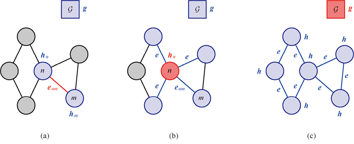
(a) edge update, (b) node update, (c) global graph update. The variable being updated is shown in red, while the variables that contribute to the update are shown in blue

Over-smoothing

“He who stays near vermilion gets red; he who stays near ink gets black.” After many rounds of message passing, all nodes become increasingly similar.

Social network rumor-spreading analogy: Imagine a rumor spreading in a social network — in the first round, your direct friends tell you some information; in the second round, information from your friends’ friends also reaches you; in the third round, the fourth round… after many rounds, everyone in the network has “heard roughly the same version”, and the original personalized information (who started the message, who it passed through in between) is completely “averaged out”. The GNN over-smoothing problem is similar: too many layers cause all node embeddings to converge to the same “average value”, losing discriminability.

• Problem: after multiple layers of message passing, node embeddings tend to become similar, limiting network depth.
• Mitigation methods:
  • Residual connection (see Part 4): $h_n^{(l+1)} = \text{Update}(...) + h_n^{(l)}$.
  • Multi-layer feature fusion: $y_n = f(h_n^{(1)} \oplus h_n^{(2)} \oplus ... \oplus h_n^{(L)})$ ($\oplus$ is concatenation).

Geometric Deep Learning

• Core: incorporate spatial symmetries (such as rotation/translation invariance of molecules) into the graph network. For example, introduce an atom coordinate embedding ($r_n^{(l)}$) in a molecule model, and use the squared coordinate difference in the update (rotation/translation invariant): $$e_{nm}^{(l+1)} = \text{Update}_{\text{edge}}(..., \|r_n^{(l)} - r_m^{(l)}\|^2)$$ ensuring that molecule property prediction is independent of the coordinate system.

Chapter 13 Summary

One-sentence version:

• Graph data: a more general structure than sequences and images — nodes (entities) + edges (relations), applicable from molecules to social networks
• Message passing: the core operation of GNNs — each round aggregates neighbor information and updates its own state, like “updating your own view by listening to your friends’ opinions”
• Aggregation operators: sum (preserves neighbor count), mean (normalized), max (captures key features), the choice depends on the task
• Permutation invariance/equivariance: graph predictions must not depend on the node index order — graph-level predictions must be invariant, node-level predictions must change synchronously with the nodes
• Graph attention: lets nodes learn “which neighbors to pay more attention to”, like trusting some friends’ opinions more in social life
• Over-smoothing: too many rounds of message passing make all node embeddings converge — mitigated by residual connections and multi-layer feature fusion

Knowledge map:

1
Graph = nodes + edges (represented by adjacency matrix)
2
    ↓ permutation invariance/equivariance constraints
3
Message passing framework: aggregate (neighbor info) → update (own state)
4
    ├── Graph convolution: neighbor aggregation with shared parameters (analogous to CNN)
5
    ├── Graph attention: dynamically weighted neighbors (analogous to Transformer attention)
6
    └── General graph network: + edge embedding + global graph embedding
7
    ↓ multi-layer stacking → over-smoothing problem → mitigated by residual connection
8
    ↓
9
Downstream tasks: node classification / edge prediction / graph classification

Thanks for reading! Follow me if you'd like~

Deep Learning Notes-6: Transformer and Graph Neural Networks

Mon Sep 01 2025

6401 words · 34 minutes

NotesDeep LearningLearningTransformerGNNGraph Neural NetworkAttention Mechanism

---

© MuxiaoWF | CC BY-NC-SA 4.0

Share

Share this article

X (Twitter)TelegramRedditFacebookEmailQQ

Close

Close