Part 5/8 of the series ← Previous | Next | Glossary

It is recommended to read Parts 1-4 first, especially the neural network basics in Part 3 and backpropagation in Part 4. This part explains how CNNs process images, and how probabilistic graphical models represent relationships between variables.

Chapter 10 Convolutional Networks

Computer Vision

Traditional machine learning models usually assume the input data is “unstructured,” meaning the elements of the input vector $\mathbf{x} = (x_1, ..., x_D)$ are mutually independent. But much of real-world data has structural features, for example:

• In natural language, words appear in sequence, with dependencies between preceding and following words.
• In images, pixels are arranged in a two-dimensional grid, and neighboring pixels are highly correlated.

If you randomly permute the pixels of an image, it no longer looks like a natural image; likewise, independently and randomly generating each pixel can almost never produce a “decent” image. This shows that images have strong local correlation and spatial structural priors.

Encode this structural prior into the model, rather than letting the model learn it from scratch. (Recall: the fully connected networks in Part 3 do not exploit this structure.)

The Convolutional Neural Network (CNN) is an architectural solution that explicitly models the spatial structure of images through sparse connectivity and parameter sharing.

Image Data

• An image is a rectangular array made up of pixels.
• Each pixel has:
• Grayscale image: single channel (intensity)
• Color image: three channels (RGB, red, green, blue)
• Pixel values are non-negative, usually represented by 8-bit integers (range 0-255).
• Video can be viewed as a three-dimensional structure (time + height + width); medical images (such as MRI) are three-dimensional voxels.

Challenge: using a fully connected network directly on images leads to an explosion of parameters.
For example: a $1000 \times 1000$ color image has 3 million dimensions (100010003=3000000) as input.
If the first layer has 1000 neurons, then just the first layer has $3 \times 10^9$ weights, which is untrainable.

Convolutional Filters

Fully connected networks have far too many parameters to process images and simply cannot be trained. The idea of CNNs is straightforward: since images have spatial structure, “hard-code” this structure into the network architecture — use sparse connectivity (each neuron only looks at a small patch) and parameter sharing (the same filter scans the entire image) to drastically reduce parameters.

CNNs exploit four structural properties of images:

1. Hierarchy: from edges → textures → parts → objects, abstracted layer by layer
2. Locality: each neuron only looks at a local region (no need to see the whole image)
3. Translation equivariance: a cat in the top-left corner and in the bottom-right corner should be detected by the same feature
4. Invariance: the final classification should not change just because the cat moved

Feature Detectors

Consider a grayscale image (single channel).

• Each hidden-layer neuron only receives a small region of the image (called the receptive field) as input.
• For example, a $3 \times 3$ receptive field corresponds to 9 inputs.
• The neuron’s output can be written as: $$z = \text{ReLU}(w^T x + w_0)$$ where:
  • $x$: the pixel vector within the receptive field.
  • $w$: the weight vector, which can be viewed as a $3 \times 3$ matrix (called a convolution kernel or filter).
  • $w_0$: the bias term.
  • $\text{ReLU}$: the activation function, defined as $\text{ReLU}(x) = \max(0, x)$.

The neuron is detecting image patches similar to the pattern of w. The more similar the input x is to w (the larger the dot product), the stronger the output response.

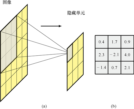
a is the receptive field, which receives a 3*3 pixel input, forming the receptive field of a hidden unit. b is the weight values associated with the hidden unit, called the convolution kernel.

Translation Equivariance

The same feature (e.g., an eye) may appear anywhere in the image. We want the same filter to detect that feature at all positions.

Solution: share weights across the entire image, i.e., slide the same convolution kernel over the image. This operation is called convolution. In practice, the “convolution” in deep learning is usually cross-correlation (computing the dot product of the filter with the input at each position).

Intuition: the convolution operation is like holding a magnifying glass and scanning the image row by row. The magnifying glass (the convolution kernel) only looks at a small region (the receptive field) at a time, then computes a single value. When the magnifying glass moves to the edge of the image, it “sees” the edge pattern and the output becomes large; when it moves to a flat region, the output is small. The same magnifying glass scans from the top-left to the bottom-right corner, finding all similar patterns across the whole image — this is the power of parameter sharing.

2D convolution formula (ignoring the activation function) $C(j, k) = \sum_l \sum_m I(j + l, k + m) \cdot K(l, m)$ where:

• $I(j, k)$: the pixel value of the input image at position $(j, k)$.
• $K(l, m)$: the weight of the convolution kernel at relative position $(l, m)$.
• $C(j, k)$: the value at position $(j, k)$ of the output feature map (the output of the convolution operation).

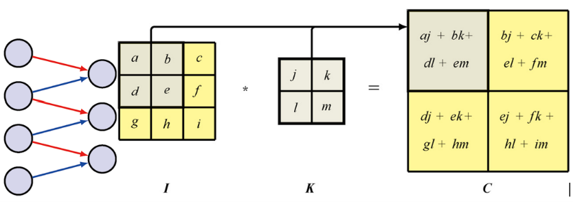
Left: 1D convolution (connections of the same color share the same weights). Right: 2D convolution.

Padding

After convolution, the feature map size shrinks. For example: a J×K image convolved with an M×M kernel produces an output of (J−M+1)×(K−M+1).

Add “padding” pixels at the edges of the image.

• Valid convolution: no padding (P=0)
• Same convolution: padding so that the output size equals the input size. When M is odd, P = (M-1)/2 The padding value is usually set to 0 (but it is recommended to mean-normalize the image first, so that 0 is close to the average pixel value).

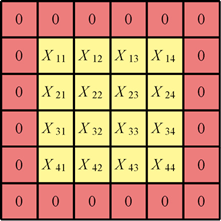
Padding

Strided Convolution

Use a stride $S > 1$, i.e., the filter moves $S$ pixels each time.

The output feature map size is controlled to be:

• J×K: the size of the input image (height × width)
• P: the padding size
• M: the convolution kernel size (assumed to be a square M×M)
• S: the stride
• $\left\lfloor \cdot \right\rfloor$: the floor function

Example:

• Input: 7×7 image, kernel: 3×3, stride: 2, padding: 1
• Output size: $\left\lfloor \frac{7 + 2×1 - 3}{2} + 1 \right\rfloor = \left\lfloor \frac{6}{2} + 1 \right\rfloor = \left\lfloor 4 \right\rfloor = 4$, so the output is 4×4

Multi-channel Convolution

The input image has multiple channels (e.g., RGB three channels), so the convolution kernel must also be three-dimensional: $M \times M \times C$, where $C$ is the number of input channels.

Use an $M \times M$ filter for each channel, then sum the results.

Input image: red, green, blue

Convolution kernel: red weights, green weights, blue weights all 3×3 = a three-dimensional kernel of 3×3×3

Extension: multiple output channels (i.e., multiple filters) Use a filter tensor of $M \times M \times C \times C_{out}$. Each output channel corresponds to an independent filter. Total number of parameters: $(M^2 \cdot C + 1) \cdot C_{out}$ (+1 is the bias, one per output channel)

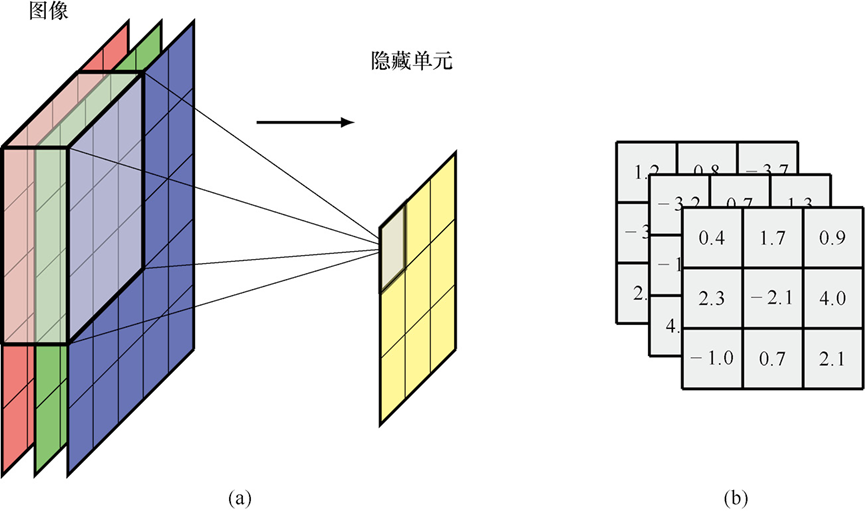
Receives input from the three RGB channels; the kernel has 27 weights (+1 bias parameter not shown).

1×1 convolution: the filter size is 1×1×C.

Effect: Change the number of channels (up-sampling or down-sampling dimensions) Introduce non-linearity (together with an activation function) Small computation cost, often used in network bottleneck layers

Reduce the number of channels to lower the computational burden, or fuse cross-channel information.

Pooling

Pooling is a down-sampling operation (reducing data resolution) in convolutional neural networks.

Intuition: pooling is like shrinking a large photo into a thumbnail. The thumbnail loses some detail, but the main features (e.g., “there is a cat here”) are still discernible. Max pooling is equivalent to “keeping only the most prominent feature,” and average pooling is equivalent to “taking the average impression of the region.” The shrunk image takes up less space and is processed faster.

Purpose: introduce translation invariance (small shifts do not affect classification). Further down-sample and reduce the feature map size. Reduce parameters and prevent overfitting (the model memorizing the training data too well).

It can be divided into max pooling (taking the maximum within the receptive field) and average pooling (taking the average).

• Pooling has no parameters; it is a fixed function.
• Usually a 2×2 window with a stride of 2 is used.
• Each channel is pooled independently.

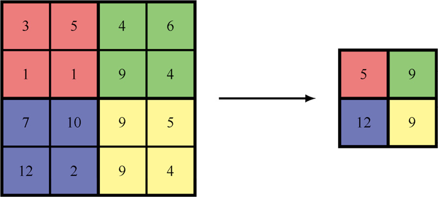
Max pooling

Multi-layer Convolution

A CNN is usually composed of multiple stacked “convolution + activation + pooling” layers.

Structure flow:

1
Input Image
2
→ Conv Layer (convolutional layer: uses multiple filters to perform convolution on the input and extract features)
3
→ Activation (activation function: usually applies a ReLU activation to non-linearly transform the convolution result)
4
→ Pooling (pooling layer: down-samples via max pooling or average pooling to reduce data dimensions)
5
→ Conv Layer (repeating structure: multiple convolutional layers, activation functions, and pooling layers stacked alternately)
6
→ Activation
7
→ Pooling
8
→ ...
9
→ Fully Connected Layers (fully connected layer: uses fully connected layers at the end of the network to integrate features)
10
→ Output

• Each layer extracts more abstract features (edges → textures → parts → objects)
• Parameter sharing and sparse connectivity drastically reduce the number of parameters
• The hierarchical structure enables the model to learn complex patterns

Advantages:

• Few parameters, easy to train
• Possesses translation equivariance and local invariance
• Can handle inputs of arbitrary size (in principle)

Through the combination of multiple layers of convolution, activation, and pooling, a CNN builds a hierarchical feature extraction system. This design not only drastically reduces the number of parameters, but also enables the network to progressively extract from low-level features to high-level semantic features.

Visualizing a Trained CNN

Understanding “what a CNN has learned” is an important question. We can explore the feature representations of different layers through visualization techniques.

Filters

An intuitive method: find the image patches in the validation set that maximize a neuron’s activation value.

• Layer 1: usually responds to edges, corners, color blobs (similar to Gabor filters). Corresponds to features detected by active neurons in the mammalian visual cortex
• Layer 2: responds to textures, simple geometric shapes.
• Layer 3: object parts start to appear (e.g., wheels, eyes, bird beaks).
• Layer 4: combinations of complex parts or local object features
• Layer 5 (high level): responds to complete objects (e.g., faces, dogs, cars).

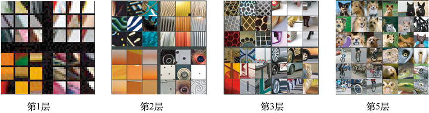
Trained filters

A more powerful method is to directly optimize the input image so as to maximize the activation of a certain neuron.

• Optimization objective: maximize the pre-activation value of some hidden unit or output unit.
• Why use pre-activation? To avoid cross-class interference introduced by softmax normalization. - Related to adversarial training (later chapters)

For example, maximizing the pre-activation value of the “dog” class output can generate an image that is “most dog-like.”

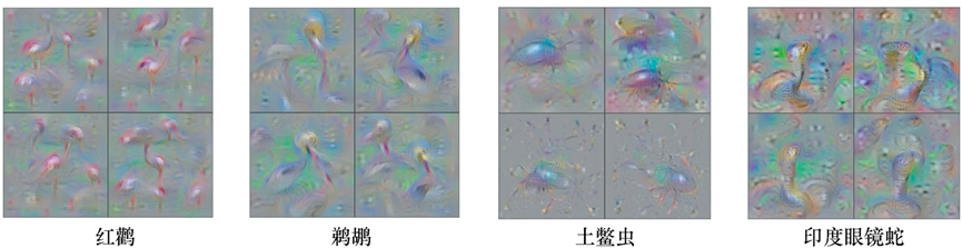
Maximize class probability to generate image

Saliency Maps

A saliency map is a visualization technique used to identify the regions in the input image that have the greatest influence on the network’s final classification decision:

• Determine the importance of each pixel by computing the gradient of the loss function with respect to the input pixels.
• A pixel with a large absolute gradient indicates that a tiny change will have a large impact on the classification result, and is therefore “salient.”

Gradient-weighted Class Activation Mapping (Grad-CAM):

1. Select the target class $c$: for example, we want to see why the network thinks this image is a “dog.”
2. Forward pass: compute the network output, obtaining the pre-activation value $a_c$ of the target class $c$ (dog).
3. Backpropagate the gradient: compute the gradient of $a_c$ with respect to the pre-activation value $a_{ij}^{(k)}$ of each neuron in the last convolutional layer. $$\frac{\partial a_c}{\partial a_{ij}^{(k)}}$$
4. Compute the weights $\alpha_k$: for each channel $k$, compute the global average of its gradients. $$\alpha_k = \frac{1}{M_k} \sum_i \sum_j \left[ \frac{\partial a_c}{\partial a_{ij}^{(k)}} \right]$$ where:

• $M_k$ is the total number of neurons in channel $k$.
• $\alpha_k$ can be understood as the “importance” of channel $k$ for the target class $c$.

5. Generate the heatmap: weight and sum the feature maps $A^{(k)}$ of the last convolutional layer by $\alpha_k$. $$L = \sum_k \alpha_k \cdot A^{(k)}$$ $L$ is the saliency heatmap, with the same size as the output of the last convolutional layer (e.g., 14×14).
6. Upsample and overlay: upsample (resize) $L$ to the size of the original image, and overlay it on the original image, using color intensity to represent saliency.

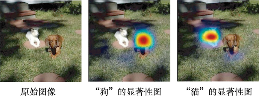
Saliency map

Adversarial Attacks

Adversarial attacks reveal a surprising weakness of deep neural networks: carefully designed, imperceptible perturbations that the human eye cannot detect can cause the network to make completely wrong classifications.

The Fast Gradient Sign Method is a simple yet effective way to generate adversarial examples:

Principle:

1. Compute the gradient: compute the gradient of the loss function $E(x, t)$ with respect to the input image $x$, $\nabla_x E(x, t)$ (the gradient computation relies on the backpropagation algorithm).

• $x$: the original image
• $t$: the true label
• $E$: e.g., negative log-likelihood

2. Generate the perturbation: the direction of the perturbation $\delta$ is the same as the gradient direction, with the goal of maximizing the loss. $$\delta = \varepsilon \cdot \text{sign}(\nabla_x E(x, t))$$

• $\varepsilon$: a very small scalar (e.g., 0.01) controlling the perturbation magnitude
• $\text{sign}()$: takes the sign of the gradient (+1 or -1)

3. Construct the adversarial example: $$x' = x + \delta = x + \varepsilon \cdot \text{sign}(\nabla_x E(x, t))$$

$\varepsilon$ must be small enough that the difference between $x'$ and $x$ is “imperceptible” to the human eye.

Why does it work?

The gradient direction is the direction of fastest increase of the loss function. Even though the network has strong generalization ability, its decision boundary can be very complex and “fragile” in high-dimensional space. A tiny, correctly-directed perturbation can push the input sample to the other side of the decision boundary.

This fragility does not stem from overfitting. Adversarial examples generated by one network can often also fool other networks with different structures.

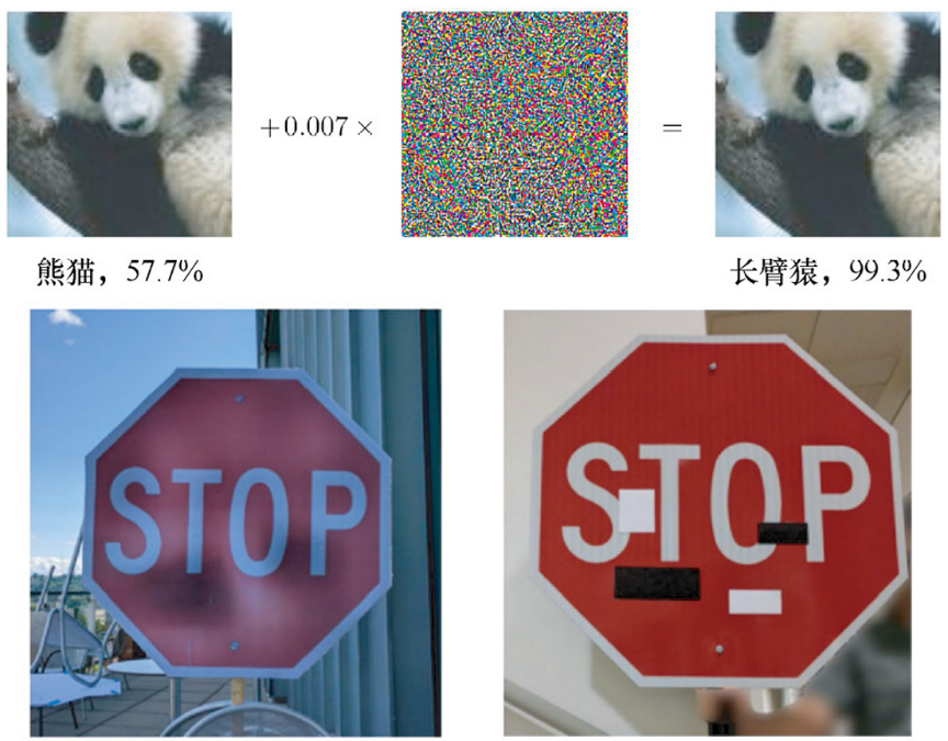
Top: a panda is recognized as a gibbon. Bottom: a stop sign is recognized as a speed limit.

Synthetic Images

The DeepDream technique: DeepDream is a technique for generating artistic images that produces surreal, dream-like images by amplifying the patterns detected by the network at specific layers.

How it works:

1. Select the target layer: choose some hidden layers of the network (usually middle layers).
2. Forward pass: feed the input image into the network and compute the activation values of all neurons in that layer, $a_{ijk}(I)$.
3. Set the backward gradient: during backpropagation, set the error signal $\delta$ of that layer to the activation values of that layer themselves. $$\delta_{ijk} = a_{ijk}(I)$$
4. Backpropagate the gradient: backpropagate the gradient into the input pixel space, obtaining $\nabla_I F(I)$.
5. Update the image: move the original image $I$ a small step along the gradient direction. $$I_{new} = I + \eta \cdot \nabla_I F(I)$$
6. Repeat: repeat steps 2-5 multiple times, and the effect becomes increasingly strong.

The whole process can be viewed as maximizing a function:

i.e., maximizing the sum of squares of the activation values of all neurons in the selected layer.

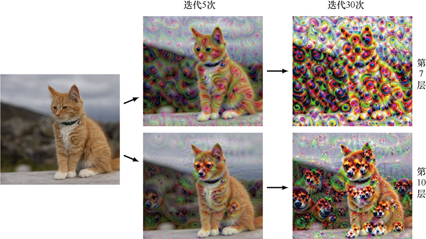
DeepDream example

Object Detection

The object detection task not only classifies objects in an image, but also localizes them (usually with bounding boxes).

Bounding Boxes

• Representation: use a rectangular box to locate an object, usually defined by four parameters: center coordinates (bx, by) and width/height (bW, bH). These values are usually normalized to the [0, 1] interval.
• Network output: on top of a standard classification network, add 4 output nodes to regress the four coordinates of the bounding box.
• Loss function:
  • Classification loss: cross-entropy is usually used.
  • Localization loss: sum-of-squares error is used to measure the discrepancy between the predicted box and the ground-truth box.

Intersection over Union (IoU)

IoU is the core metric for evaluating the localization accuracy of an object detection model.

• Definition: the area of intersection of the predicted bounding box and the ground-truth bounding box divided by the area of their union.
• Range: [0, 1]. The larger the value, the higher the overlap between the two boxes, and the more accurate the localization.
• Criterion: a prediction with IoU ≥ 0.5 is usually considered a “correct detection.”

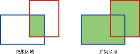
Green on the left is larger than green on the right.

Sliding Window

The naive sliding window method is extremely inefficient, because a complete network forward pass must be performed independently for each window position, and the inputs of adjacent windows are highly overlapping, causing a lot of redundant computation in the convolutional layers.

Fully convolutional idea: feed the entire large image into a Fully Convolutional Network (FCN) at once.

• Principle: a convolution operation is essentially the weight-sharing version of a sliding window. When the input image becomes larger, the convolutional layer naturally applies the filter at all possible positions, outputting a feature map where each position corresponds to the response of a receptive field in the original image.
• Result: a single forward pass yields the classification results for all window positions, greatly improving efficiency.

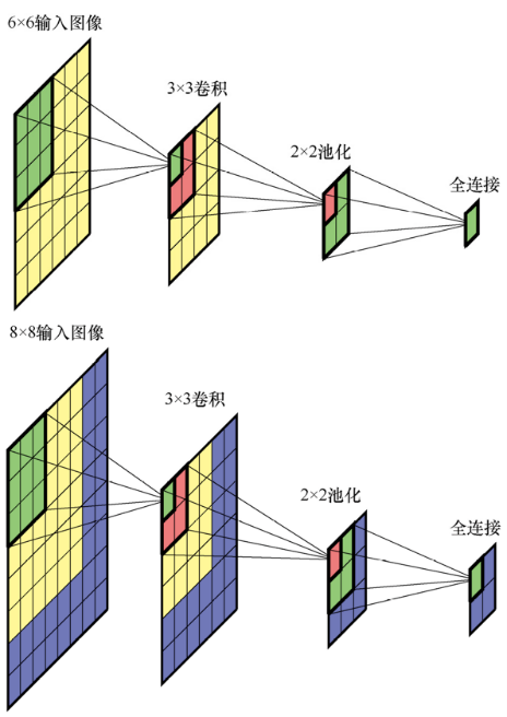
Top vs. bottom comparison: the only extra computation is the blue part.

Image Segmentation

Image segmentation is a finer task than object detection: assign a category label to every pixel in the image.

Convolutional Segmentation

Naive Method

• Take a local window centered on each pixel as input.
• Feed it into a CNN to classify that pixel.
• Repeat this for all pixels.

A lot of redundant computation, extremely inefficient.

Improved Method: Fully Convolutional Network (FCN)

• Replace the fully connected layers of a traditional CNN with convolutional layers.
• The entire network consists of convolution, pooling, and activation.
• Input an arbitrary-size image → output a segmentation map of the same spatial size.

A single forward pass yields predictions for all pixels, which is efficient.

Upsampling

Pooling reduces the resolution of the feature map, losing spatial information.

Use up-sampling or transposed convolution to restore the low-resolution feature map to the original image size.

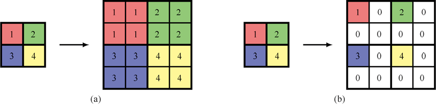
Left: corresponds to average pooling. Right: corresponds to max pooling (the max position can also be recorded and restored).

Transposed Convolution

Can “enlarge” a small feature map into a large feature map, and can be viewed as the “reverse” process of convolution.

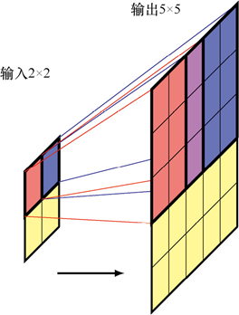
Transposed convolution (overlapping parts can be summed or averaged).

Fully Convolutional Network (FCN)

• The FCN architecture does not use pooling; that is, FCN replaces fully connected layers with 1×1 convolutions, and all up- and down-sampling is done by convolutions.
• Advantages:
  • Can handle arbitrary-size inputs
  • Output is a segmentation map of the same size
  • Parameter sharing, efficient

Role of 1×1 convolution: change the number of channels without changing the spatial size (often used to reduce the number of channels to the number of classes C).

U-Net Architecture

U-Net is a classic architecture for semantic segmentation.

• Encoder (downsampling path): a series of convolutions + pooling that extracts high-level semantic features, but reduces resolution.
• Decoder (upsampling path): a series of upsampling + convolution that progressively restores spatial resolution.
• Skip connections: directly “skip” the feature map of a certain encoder layer and concatenate it to the input of the corresponding decoder layer.

This “passes” the high-resolution detail information of low layers to high layers, compensating for the spatial information loss caused by pooling.

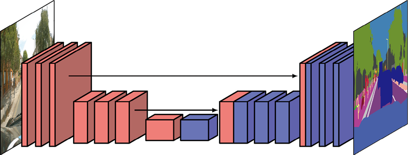
U-Net has a symmetric arrangement of downsampling and upsampling layers; the output of each downsampling layer is concatenated to the corresponding upsampling layer.

Style Transfer

Neural style transfer is an artistic image generation technique that combines the “content” of one image with the “style” of another.

Basic idea:

• Content image (C): provides the scene and objects (e.g., a photo).
• Style image (S): provides the artistic style (e.g., a Van Gogh painting).
• Generated image (G): a synthesized image whose content looks like C and style looks like S.

The total loss function (one term similar to the original content, one term similar to the original style):

Treat the generated image $G$ as a learnable parameter, initialized from the content image $C$ or from random noise, and minimize the total loss $E(G)$ via gradient descent, so that the generated image $G$ looks like $C$ in high-level semantics, and like $S$ in texture, brushstrokes, and color distribution.

Select an intermediate convolutional layer (usually one that captures object contours), and compute the squared error of the feature activations of $G$ and $C$ at that layer (content loss):

where $a_{ijk}(I)$ is the pre-activation value of the input image $I$ at position $(i,j)$ and channel $k$.

• Content image C activations at layer 10: [0.8, 0.2, 0.9, …]
• Generated image G activations at layer 10: [0.7, 0.3, 0.8, …]
• Content loss = (0.8-0.7)² + (0.2-0.3)² + (0.9-0.8)² + …

To ensure that the generated image $G$ is similar in style to the style image $S$, the correlation between different feature channels must be maintained, using the style matrix:

For the selected convolutional layer, compute its style matrix $F$:

$F_{kk'}$ measures the spatial co-occurrence (correlation) degree of features of channels $k$ and $k'$.

The style loss is the squared error between the style matrices of $G$ and $S$:

Usually a weighted sum of the style losses of multiple layers is used, to capture style features at different scales:

Chapter 10 Summary

One-sentence version: A CNN scans an image with convolution kernels (sparse connectivity + parameter sharing) to extract hierarchical features from edges to objects, uses pooling to reduce dimensions, then uses fully connected layers for classification; it can also be visualized, be fooled (adversarial attacks), and can perform detection, segmentation, and style transfer.

Knowledge map:

• Why CNNs are needed: images have spatial structure; fully connected networks have an explosion of parameters
• Core operations: convolution (feature extraction) -> activation (ReLU) -> pooling (dimension reduction) -> multi-layer stacking
• Key concepts: receptive field, convolution kernel/filter, padding, stride, parameter sharing, translation equivariance
• What CNNs can do: classification, object detection (bounding box + IoU), image segmentation (FCN + U-Net), style transfer
• Understanding CNNs: filter visualization, saliency maps, Grad-CAM
• CNN’s weakness: adversarial attacks (tiny perturbations cause misclassification)

Want to know how gradients in a CNN are computed? Please review backpropagation in Part 4. Want to see how CNNs are replaced by Transformers in modern architectures? Please continue to Part 6.

Chapter 11 Structured Distributions

Probabilistic Graphical Models

The core idea of Probabilistic Graphical Models (PGM) is intuitive: use a connection graph to represent the causal and dependency relationships between variables. Just as a circuit diagram in engineering uses boxes and connections to represent the wiring between components, a probabilistic graphical model uses nodes (boxes) to represent random variables and arrows (connections) to represent “who influences whom.” With a glance at the graph, you can tell which variables are dependent and which are independent — without any mathematical derivation.

All probability operations are essentially built on two basic rules:

• Sum rule: $p(X) = \int p(X, Y) dY$ (marginalize to get the marginal distribution)
• Product rule: $p(X, Y) = p(Y|X)p(X)$ (get the joint distribution)

Although we could handle complex probabilistic models using algebra alone, using a graphical representation has huge advantages:

1. Visualize structure: intuitively show the dependencies of a probabilistic model, helping to design and understand new models.
2. Reveal properties: by observing the structure of the graph, one can infer the conditional independence between variables.
3. Simplify computation: complex inference and learning algorithms (such as message passing) can be expressed as operations on the graph, making the underlying mathematics clearer.

Note: After this point, neural network graphs are shown in blue, while probabilistic graphical models are shown in red, to avoid confusion.

Directed Graphs

A directed graphical model (also called a Bayesian network or Bayes net) is a type of probabilistic graphical model in which the edges (links) carry arrows, indicating dependencies or causal relationships between variables. Its basic elements are:

• Nodes (Vertices): represent random variables (e.g., $a$, $b$, $c$).
• Directed edges (Links): an arrow points from one variable to another, indicating that the former is the “cause” or “parent” of the latter.
• Parent and child nodes: if there is an arrow from $a$ to $c$, then $a$ is the parent of $c$, and $c$ is the child of $a$.

It should be noted that although the edges in a Bayesian network have directions, this does not always mean causality. The direction of an edge more represents the dependency relationship between variables and the order of factorization.

Factorization

Consider the joint distribution $p(a, b, c)$ of three variables $a$, $b$, $c$.

By the product rule, it can be factorized:

Graphical Representation

We can draw the above factorization as a directed graph:

• Create a node for each variable $a$, $b$, $c$.
• Add a directed edge for each conditional probability factor:
  • $p(c | a, b)$: draw arrows from $a$ and $b$ pointing to $c$.
  • $p(b | a)$: draw an arrow from $a$ pointing to $b$.
  • $p(a)$: no condition, so no edge points to $a$.

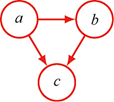
Factorization graph

Fully connected graph: for K variables, the most general factorization is: $p(x_1, ..., x_K) = p(x_K | x_1, ..., x_{K-1}) \cdot ... \cdot p(x_2 | x_1) \cdot p(x_1)$ The corresponding graph is a fully connected graph: each node receives edges from all nodes with smaller indices.

• This factorization applies to any joint distribution.
• But such a graph provides no “interesting” information, because it assumes all variables may depend on each other.

The truly valuable information comes from the missing edges. Because the presence of an edge represents a direct dependency (given the parents). And therefore the absence of an edge represents a conditional independence.

For a directed graph with K nodes, the general factorization rule for its joint probability distribution is:

where:

• $pa(k)$ denotes the parent set of node $x_k$ (parents of k).
• The product is taken over all nodes in the graph.
• As long as each conditional probability $p(x_k | pa(k))$ is normalized (i.e., integrates to 1 over $x_k$), then the whole product is automatically normalized.

Discrete Variables

When the nodes in a graphical model represent discrete variables, each variable has $K$ possible states (e.g., $K$ categories).

The distribution of a $K$-state discrete variable $x$ is defined by a parameter vector $\mu = (\mu_1, ..., \mu_K)^T$, satisfying $\sum_{k=1}^K \mu_k = 1$. Its probability mass function is:

where $x_k \in \{0,1\}$ is the one-hot encoding of $x$, i.e., only one $x_k=1$ and the rest are 0. Due to the normalization constraint, only $K-1$ parameters need to be specified.

Consider two discrete variables $x_1$ and $x_2$, each with $K$ states.

• Full joint distribution: $p(x_1, x_2)$ is defined by $K^2$ values $\mu_{kl} = p(x_1=k, x_2=l)$. Since $\sum_{k,l} \mu_{kl} = 1$, the number of independent parameters is $K^2 - 1$.
• Chain structure: using the product rule, $p(x_1, x_2) = p(x_2|x_1)p(x_1)$.
  • $p(x_1)$ needs $K-1$ parameters.
  • $p(x_2|x_1)$ needs $K(K-1)$ parameters (because for each of the $K$ values of $x_1$, $p(x_2|x_1)$ is a $K$-state distribution needing $K-1$ parameters).
  • Total parameters: $(K-1) + K(K-1) = K^2 - 1$, the same as the full joint distribution.

A fully connected directed graph (e.g., an arrow from $x_1$ to $x_2$) can represent any joint distribution, because it imposes no restriction.

Relationship Between Number of Parameters and Graph Structure

• Fully connected graph (all possible edges exist): can represent the most general joint distribution, but the number of parameters is $K^M - 1$, growing exponentially with the number of variables $M$.
• Unconnected graph (independent variables): the joint distribution is $p(x_1,...,x_M) = \prod_{i=1}^M p(x_i)$. Each $p(x_i)$ needs $K-1$ parameters, so the total number of parameters is $M(K-1)$, growing linearly with $M$.
• Partially connected graph: strikes a balance between fully general and fully independent. For example, the chain structure: $$p(x_1,...,x_M) = p(x_1)\prod_{i=2}^M p(x_i|x_{i-1})$$
  • $p(x_1)$: $K-1$ parameters.
  • Each $p(x_i|x_{i-1})$: $K(K-1)$ parameters.
  • Total parameters: $K-1 + (M-1)K(K-1)$, growing linearly with the chain length $M$ (rather than exponentially), but able to represent more complex dependencies than the independent model.

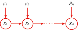
Partially linked graph (chain structure) reduces parameters

A further way to reduce parameters is parameter sharing.

In a chain structure, we can assume that all the conditional distributions $p(x_i|x_{i-1})$ ($i=2,...,M$) are controlled by the same set of $K(K-1)$ parameters.

• Effect: the total number of parameters becomes $K-1 + K(K-1)$, independent of $M$.
• Limitation: this means all transitions (from $x_{i-1}$ to $x_i$) follow the same “rule.”
• Application: this is common in Hidden Markov Models (HMM) and Recurrent Neural Networks (RNN).

Similar to the figure above, but the topmost parameter $\mu$ can be shared by multiple nodes in the graphical model.

Gaussian Variables

Conditional distributions:

Consider an arbitrary directed acyclic graph with $D$ variables, where node $i$ represents a single continuous random variable $x_i$ with a Gaussian distribution. The mean of this distribution is taken as a linear combination of the states of the parent nodes $\text{pa}(i)$:

where:

• $w_{ij}$ and $b_i$ are the parameters controlling the mean,
• $v_i$ is the variance of the conditional distribution $x_i$.

Joint distribution:

The log of the joint distribution is the product of the logs of all node conditional distributions:

Substituting the above gives:

where $\mathbf{x} = (x_1, \dots, x_D)^T$, and ‘const’ denotes terms independent of $\mathbf{x}$.

This expression is a quadratic function of the components of $\mathbf{x}$, so the joint distribution $p(\mathbf{x})$ is a multivariate Gaussian distribution.

• The mean of each variable satisfies the following recurrence relation:

  $$\mathbb{E}[x_i] = \sum_{j \in \text{pa}(i)} w_{ij} \mathbb{E}[x_j] + b_i$$

  Assuming the node indices are such that each node has a higher index than its parents, one can start from the smallest-indexed node and recursively compute each component of $\mathbb{E}[\mathbf{x}] = (\mathbb{E}[x_1], \dots, \mathbb{E}[x_D])^T$.

• The covariance matrix elements of the joint distribution satisfy the recurrence relation:

  $$\text{cov}[x_i, x_j] = \sum_{k \in \text{pa}(j)} w_{jk} \text{cov}[x_i, x_k] + I_{ij} v_j \quad (11.13)$$

  where $I_{ij}$ is an indicator function (1 when $i = j$, 0 otherwise). The covariance can also be computed recursively starting from the smallest-indexed node.

Consider a joint Gaussian distribution whose covariance matrix is partially constrained: $x_1 \to x_2 \to x_3$

• Mean:

  $$\mathbf{\mu} = (b_1, \, b_2 + w_{21}b_1, \, b_3 + w_{32}b_2 + w_{32}w_{21}b_1)^T$$

• Covariance matrix:

  $$\mathbf{\Sigma} = \begin{pmatrix} v_1 & w_{21}v_1 & w_{32}w_{21}v_1 \\ w_{21}v_1 & v_2 + w_{21}^2 v_1 & w_{32}(v_2 + w_{21}^2 v_1) \\ w_{32}w_{21}v_1 & w_{32}(v_2 + w_{21}^2 v_1) & v_3 + w_{32}^2(v_2 + w_{21}^2 v_1) \end{pmatrix}$$

Similarly, the linear-Gaussian graphical model can be extended to the case where nodes represent multivariate Gaussian variables. The conditional distribution of node $i$ is:

where $\mathbf{W}_{ij}$ is a matrix (non-square if $\mathbf{x}_i$ and $\mathbf{x}_j$ have different dimensions). It is likewise easy to verify that the joint distribution of all variables is still Gaussian.

Model Representation

In practical applications, when we use graphical models for machine learning problems, we usually set some random variables to specific observed values. For example, in a linear regression model, the random variable ${t_n}$ would be set to the concrete values in the training set. In a graphical model, we represent these observed variables by shading the corresponding nodes.

In addition, model parameters (such as the weight $w$) are usually treated as deterministic parameters, represented by floating variables. Unobserved random variables (such as latent or hidden variables) are represented by open red circles.

Ultimately, we have three kinds of variables:

1. Unobserved random variables (latent variables), represented by open red circles.
2. Observed random variables, represented by blue-shaded red circles.
3. Non-random parameters, represented by floating variables.

This representation helps clearly describe the structure of the model and the relationships between variables, providing a basis for subsequent inference and learning.

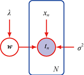
Example graph

• Red circle $w$: represents the model’s parameter (weight), i.e., a non-random variable. In the graph it is represented by a “floating variable,” indicating it is a learnable parameter rather than a random variable.
• Blue rectangle $N$: indicates there are $N$ identical nodes.
• Red circle $t_n$: shaded blue, indicating this is an observed variable (i.e., the true label in the training data). In probabilistic graphical models, observed variables are represented by shaded nodes.
• $x_n ,\sigma^2,\lambda$: floating variables, deterministic parameters.

Conditional Independence

Consider three random variables $a$, $b$, and $c$. If, conditioned on $c$, the conditional distribution of $a$ does not depend on the value of $b$, i.e.:

then we say $a$ is conditionally independent of $b$ given $c$ (conditional independence).

This can also be expressed through the joint distribution. Using the product rule of probability:

Substituting conditional independence into the above gives:

This shows that, conditioned on $c$, the joint distribution of $a$ and $b$ can be factorized into the product of their respective conditional distributions, i.e., $a$ and $b$ are statistically independent given $c$.

For concise notation, we use the following symbol:

to indicate that $a$ is conditionally independent of $b$ given $c$.

Note: conditional independence must hold for all possible values of $c$, not just some specific values.

Three Examples

Directly verifying conditional independence through probability calculations is very time-consuming. The advantage of graphical models is that we can directly judge from the graph structure which variables are conditionally independent. This method is called d-separation (d stands for “directed”).

Understand it through three simple three-node graph examples:

1. Graph structure: a → c ← b The corresponding joint distribution is: $$p(a, b, c) = p(a|c)p(b|c)p(c)$$

• When no variable is observed, marginalizing over $c$: $$p(a, b) = \sum_c p(a|c)p(b|c)p(c)$$ This generally cannot be factorized as $p(a)p(b)$, so $a$ and $b$ are not independent, written as $a \not\perp\!\!\!\perp b \mid \emptyset$.
• When $c$ is observed (i.e., conditioning on $c$), the joint distribution becomes: $$p(a, b|c) = \frac{p(a, b, c)}{p(c)} = p(a|c)p(b|c)$$ At this point $a$ and $b$ are independent given $c$, i.e., $a \perp\!\!\!\perp b \mid c$.
• Node $c$ in the path $a \to c \leftarrow b$ is tail-to-tail (arrow tails connected). When $c$ is not observed, the path is “open” (information can pass along this path, so there is a dependency between the variables), and $a$ and $b$ are dependent; when $c$ is observed (conditioned on), the path is “blocked,” and $a$ and $b$ become conditionally independent.

  When c is not observed: the path is “open,” and a and b are associated through the common “effect” c.

  • Example: a=rain, b=sprinkler, c=ground wet: although rain and sprinkler are unrelated, they can both cause the ground to be wet, so through the common result “ground wet,” a and b become correlated.

  After observing c: the path is “blocked”; once the state of c is known, a and b become independent.

  • Example: if we already know the ground is wet, then rain and sprinkler are independent.

2. Graph structure: a → c → b The corresponding joint distribution: $$p(a, b, c) = p(a)p(c|a)p(b|c)$$

• When no variable is observed, $a$ and $b$ are not independent (there is a path from $a$ to $b$).
• When $c$ is observed, using Bayes’ theorem: $$p(a, b|c) = \frac{p(a)p(c|a)p(b|c)}{p(c)} = p(a|c)p(b|c)$$ Therefore $a \perp\!\!\!\perp b \mid c$.
• Node $c$ in the path $a \to c \to b$ is head-to-tail (one arrow head, one arrow tail). When not observed the path is “open,” and when observed the path is “blocked.”

3. Graph structure: a → c ← b The corresponding joint distribution: $$p(a, b, c) = p(a)p(b)p(c|a, b)$$

• When no variable is observed, marginalizing over $c$: $$p(a, b) = p(a)p(b)$$ So $a$ and $b$ are independent, i.e., $a \perp\!\!\!\perp b \mid \emptyset$.
• When $c$ is observed: $$p(a, b|c) = \frac{p(a)p(b)p(c|a, b)}{p(c)}$$ This expression generally cannot be factorized as $p(a|c)p(b|c)$, so $a \not\perp\!\!\!\perp b \mid c$.
• Node $c$ in the path $a \to c \leftarrow b$ is head-to-head (arrow heads connected), also called a collider . When not observed, the path is “blocked,” and $a$ and $b$ are independent; once $c$ is observed, the path is “opened,” and $a$ and $b$ become dependent.

Not only $c$ itself, but if any descendant node of $c$ is observed, the path is also “opened.”

Take medical diagnosis as an example, considering the variables: Symptom (S), Disease (D), and Test (T).

• For the structure S→D←T: without knowing the disease, the symptom and the test result are correlated; but once the disease diagnosis is known, the symptom and the test result become independent.
• For the structure S→D→T: without knowing the disease, the symptom and the test result are correlated; once the disease is known, the two become independent.
• For the structure S→D←T: without knowing any information, the symptom and the test result are independent; but once the disease is known, the two become correlated.

d-separation

Judge whether variables are conditionally independent by checking whether the path is “open.”

Given a Directed Acyclic Graph (DAG), determine whether set $A$ is d-separated from set $B$ given set $C$:

1. Consider all paths from any node in $A$ to any node in $B$.
2. A path is “blocked” if and only if there is a node on the path that satisfies any of the following conditions:

• The node is tail-to-tail or head-to-tail, and this node is in set $C$ (i.e., observed).
• The node is head-to-head, and this node together with all its descendant nodes are not in set $C$.

3. If all paths are blocked, then $A$ is d-separated from $B$ by $C$, i.e., $A \perp\!\!\!\perp B \mid C$ holds.

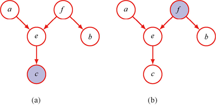
d-separation

• (a) The path from a to b is neither blocked by f (tail-to-tail and unobserved) nor by e (head-to-head but with only one observed descendant node), so $a \perp\!\!\!\perp b \mid c$ cannot be concluded.
• (b) The path from a to b is blocked by f (tail-to-tail and observed), so $a \perp\!\!\!\perp b \mid f$, and also blocked by e (head-to-head and neither it nor its descendants are observed).

Explaining Away

The head-to-head structure leads to an interesting phenomenon called “explaining away.”

Example: consider a car fuel system containing three binary variables:

• $B$: battery state (1=charged, 0=dead)
• $F$: fuel tank state (1=full, 0=empty)
• $G$: fuel gauge reading (1=full, 0=empty)

Fuel tank example

Assume $B$ and $F$ are independent, and $G$ depends on $B$ and $F$ (the gauge may read empty because the battery is dead or the tank is empty).

• Prior: $p(F=0) = 0.1$
• After observing $G=0$ (gauge empty), compute the posterior:

The probability that the tank is empty rises (from 0.1 to 0.257).

• After further observing $B=0$ (battery dead):

The probability that the tank is empty drops.

Explanation: observing that the battery is dead ($B=0$) provides an “explanation” for the gauge being empty ($G=0$), thereby “eliminating” the need for the empty tank ($F=0$) as an explanation. This shows that $B$ and $F$, which were originally independent, become dependent after observing their common “effect” $G$. This is the typical behavior of a head-to-head structure.

Naive Bayes

Naive Bayes is a classification model based on the conditional independence assumption.

Assume the input vector $\mathbf{x} = (x^{(1)}, ..., x^{(L)})$, and the class is $C_k$. Its core assumption is: conditioned on the class $C_k$, the features $x^{(l)}$ are mutually independent, i.e.:

The class node $C_k$ points to all feature nodes $x^{(1)}, ..., x^{(L)}$. Since $C_k$ is a tail-to-tail node, once conditioned on $C_k$, all paths between any $x^{(i)}$ and $x^{(j)}$ are blocked, so they are conditionally independent.

For classification, use Bayes’ theorem:

where $p(\mathbf{x}) = \sum_k p(\mathbf{x}|C_k)p(C_k)$.

Note: although the conditional independence assumption is strong (in reality features are often correlated), Naive Bayes performs well on tasks such as text classification, because the decision boundary is insensitive to the details of the class-conditional densities.

Generative Models

Generative models attempt to learn the data generation process. An example of image generation:

• Class, position, and scale are independently sampled from a prior distribution.
• The image is generated from a conditional distribution that depends on class, position, and scale.
• When the image is unobserved, class, position, and scale are mutually independent (the path is head-to-head and the image is unobserved, so the path is blocked).
• After the image is observed, these variables become dependent (the path is opened). For example, knowing the object’s class helps infer its position.

Generative models can generate new samples, whereas discriminative models (such as directly trained classifiers) usually cannot.

Markov Blanket

For a node $x_i$ in a graph, its Markov blanket is the smallest set of nodes such that $x_i$ is conditionally independent of all the remaining nodes in the graph given that set.

Specifically, the Markov blanket of $x_i$ contains:

• Parent nodes
• Child nodes
• Other parent nodes of the child nodes

In a head-to-head structure, observing the child node opens the path between its parent nodes (explaining away). Therefore, to “isolate” $x_i$, one must observe both its child nodes and the other parent nodes of those children.

The Markov blanket gives the set of variables that are actually depended upon when computing $p(x_i | \mathbf{x}_{\backslash i})$, greatly simplifying inference.

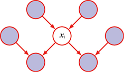
Markov blanket

Graphs as Filters

A graphical model can be understood from two equivalent perspectives:

1. Factorization perspective: the graph defines that the joint distribution must factorize into a product of conditional probabilities of a specific form.
2. Independence perspective: the graph defines, through d-separation, a set of conditional independencies that must be satisfied.

The d-separation theorem guarantees that these two perspectives are equivalent: a distribution passes the “factorization filter” if and only if it passes the “independence filter.”

We can view the graphical model (here a directed graphical model) as a kind of filter, where a probability distribution p(x) can only pass through the filter if it satisfies the directed factorization property. Let DF denote the set of all possible probability distributions p(x) that pass through the filter. We can also use the graph (as a second filter) to filter distributions based on whether they satisfy all the conditional independencies implied by the graph’s d-separation property. The d-separation theorem states that the same set of distributions DF will be allowed through the second filter.

Sequence Models

In many machine learning applications, data appears in the form of sequences. For example:

• Text is a sequence of words
• Proteins are sequences of amino acids
• Audio signals are sampled sequences over time
• Daily rainfall is a series of daily measurements

Although some sequences are not strictly time series, the terms “time,” “past,” and “future” are usually borrowed to describe the ordering relationships.

We use $x_1, \dots, x_N$ to denote a sequence of length $N$, where each $x_n$ is a vector (which can be a scalar or a multi-dimensional vector).

Sometimes we independently draw multiple such sequences from the same distribution. In that case, the joint distribution of all sequences factorizes into the product of the individual sequence distributions. In this section we mainly focus on modeling a single sequence.

General Autoregressive Models

The core idea of an autoregressive model is: use the variable’s own past values to predict the current value. By the product rule of probability, the joint distribution of any $N$ variables can be written as a product of a series of conditional distributions. If we order the variables according to the natural order of the sequence, then:

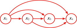
General autoregressive model, each node receives a connection from the preceding node in the sequence.

This representation is completely general, so it brings no advantage in terms of modeling, because it introduces no assumption or simplification.

To simplify the model, we can introduce conditional independence assumptions, by removing edges from the graph, or equivalently, by deleting some variables from the conditional variables on the right-hand side of formula (11.42).

The most extreme simplification is to remove all conditional variables, yielding:

This means all variables are mutually independent, completely ignoring the order information.

A more reasonable assumption is: each variable depends only on the one preceding it (first-order Markov model). In this case the joint distribution is:

First-order Markov chain

Using the d-separation criterion, it can be verified that:

This means that to predict the next observation, only the previous observation needs to be known, independent of the earlier history.

We can extend the model so that each variable depends on the previous two variables, yielding the second-order Markov model:

Second-order Markov

In general, the conditional distribution of an M-th order Markov chain depends on the previous M variables.

Number of Parameters Issue

Assume the observed variables are discrete, with $K$ states.

• First-order Markov model: the conditional distribution $p(x_n | x_{n-1})$ has $K(K - 1)$ parameters.
• M-th order Markov model: the conditional distribution $p(x_n | x_{n-M}, \dots, x_{n-1})$ has $K^{M-1}(K - 1)$ parameters.

The number of parameters grows exponentially with $M$, so higher-order models become impractical for large $M$.

• First-order model needs 10×(10-1) = 90 parameters
• Second-order model needs 10×10×(10-1) = 900 parameters
• Third-order model needs 10³×(10-1) = 9000 parameters

Latent Variable Models

To build a sequence model that is not limited by the Markov order but still has a bounded number of parameters, one can introduce latent variables (variables that cannot be directly observed but influence the observations).

For each observation $x_n$, introduce a corresponding latent variable $z_n$ (whose type or dimension may differ from $x_n$). Assuming these latent variables form a Markov chain yields a state-space model.

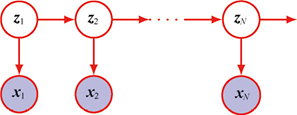
Latent variable model

• The latent variables $z_n$ form a Markov chain, meaning that given the current state $z_n$, the future state is independent of the past state.
• Each observation $x_n$ depends only on its corresponding latent variable $z_n$, not directly on other observations or latent variables.

The key conditional independence is:

The joint distribution is:

Using d-separation, one can find that any two observation variables $x_n$ and $x_m$ are connected through the latent variable path, and this path is never blocked. Therefore, the predictive distribution:

has no conditional independence, i.e., the future prediction depends on all past observations.

In other words, the observation variables themselves do not satisfy any order of the Markov property.

Chapter 11 Summary

One-sentence version: Probabilistic graphical models draw a dependency graph between variables using nodes and arrows, and through the d-separation rule one can directly tell from the graph which variables are conditionally independent, without complex probability calculations.

Knowledge map:

• Core idea: use a graph to represent the structure of a probability distribution (two equivalent perspectives: factorization + independence)
• Directed graphical model (Bayesian network): joint distribution = product of each node’s conditional probability; absence of an edge = conditional independence
• Key concepts: parent/child nodes, conditional independence, d-separation (tail-to-tail / head-to-tail / head-to-head)
• head-to-head (collider): blocks the path when unobserved, opens the path when observed (explaining away)
• Application models: Naive Bayes (classification), generative models, sequence models
• Sequence modeling: autoregressive -> Markov model (exponential growth of parameters) -> latent variable model (bounded parameters + long-term dependencies)

The “factorization” idea in probabilistic graphical models has something in common with the hierarchical structure of neural networks in Part 3 — both use structured design to reduce parameters and improve efficiency. And the latent variable idea in sequence models will reappear in the form of “attention mechanisms” in the Transformer of Part 6.

Thanks for reading! Follow me if you'd like~

Deep Learning Notes - 5: Convolutional Networks and Probabilistic Graphical Models

Mon Sep 01 2025

7931 words · 41 minutes

NotesDeep LearningLearningCNNConvolutional Neural NetworkProbabilistic Graphical Models

---

© MuxiaoWF | CC BY-NC-SA 4.0

Share

Share this article

X (Twitter)TelegramRedditFacebookEmailQQ

Close

Close