Part 4/8 of the series ← Previous | Next | Glossary

It is recommended to read Parts 1-3 first, especially the error function and regularization concepts in Part 1. This part covers how neural networks are trained (gradient descent + backpropagation) and how to prevent overfitting (regularization).

Chapter 7 Gradient Descent

Intuition first — imagine you are standing on a large mountain shrouded in dense fog, unable to see anything. You want to get down to the valley (the point of minimum error). What do you do? You feel the slope under your feet with your foot — and take a step in whichever direction is lower. By repeating this, you will eventually reach the bottom of the valley. This is the core idea of gradient descent (Gradient Descent, an optimization algorithm that minimizes the error by iteratively updating parameters along the direction of steepest error decrease).

For gradient-related material, it is recommended to study “Introduction to Optimization”. Well, I myself only managed to learn the basics of the first few chapters (lol)

Error Surface

Our goal is to find a set of parameter vectors $\mathbf{w}$ (a vector consisting of weights and biases, which can be thought of as the network’s “knobs”) such that the error function $E(\mathbf{w})$ (a function measuring the gap between the network’s predictions and the true values) is minimized. We can imagine $E(\mathbf{w})$ as a “topographic map”, where the horizontal axis is the high-dimensional weight space and the vertical axis is the error value. At any point on the mountain, you can feel the “slope” under your feet — this is the gradient (Gradient, the direction and magnitude of the fastest change of a function at a given point).

• At any point $\mathbf{w}_C$, the gradient of the error function $\nabla E(\mathbf{w}_C)$ points in the direction of fastest error increase (i.e., the “uphill” direction).
• To reduce the error, we should update the weights along the opposite direction of the gradient (i.e., “downhill”): $$\Delta \mathbf{w} = -\eta \nabla E(\mathbf{w})$$ where $\eta > 0$ is the learning rate (Learning Rate, a hyperparameter controlling how far to step at each iteration). The learning rate is like your “step size” — too large and you may leap across the valley onto the opposite mountain (diverging); too small and you walk too slowly and give up before reaching the bottom.

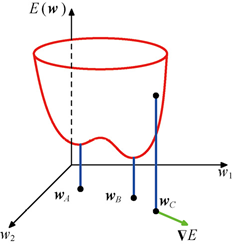
Local minimum (wA), global minimum (wB), and how the gradient direction (∇E) guides the update direction

When the gradient is zero ($\nabla E(\mathbf{w}) = 0$), we have reached a stationary point (Stationary Point, a point where the gradient is zero), which may be a local minimum, a local maximum, or a saddle point (Saddle Point, a point that is a minimum in one direction and a maximum in another, shaped like a saddle). Ideally, we want to find the global minimum, but in practice we are often content with a good local minimum.

Local Quadratic Approximation

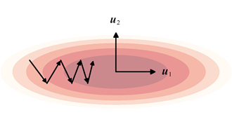
Near a minimum, the contour lines of equal error are ellipses, whose principal axes are determined by the Hessian eigenvectors

Gradient Descent Optimization

Because the error function of a neural network is extremely complex (with parameter counts often in the millions), we cannot directly solve the equation $\nabla E(\mathbf{w}) = 0$, and must use iterative numerical methods (Iterative Numerical Method, a method that gradually approaches the optimal solution by repeatedly updating parameters).

General iterative formula:

where $\tau$ denotes the iteration step (Iteration, each parameter update counts as one step).

Use of Gradient Information

Gradient information can significantly improve optimization efficiency. The reasons are as follows:

• Without using the gradient: requires $O(W^2)$ function evaluations ($W$ being the number of parameters), each evaluation being $O(W)$, for a total cost of $O(W^3)$.
• Using the gradient: each gradient evaluation provides $W$ pieces of information, so in theory $O(W)$ evaluations are enough to locate the minimum. Combined with efficient backpropagation ($O(W)$ ), the total cost drops to $O(W^2)$.

Therefore, the gradient is the foundation of training neural networks.

Batch Gradient Descent (Steepest Descent)

The simplest form of gradient descent, which uses the entire training set to compute the gradient:

where $E(\mathbf{w}) = \sum_{n=1}^N E_n(\mathbf{w})$ is the error over the full dataset. Each update requires iterating over all the data, which is computationally expensive.

Stochastic Gradient Descent (SGD)

Intuition: Batch gradient descent is like wanting to survey the average height of people across the whole country — you have to ask everyone, which is too slow. Stochastic gradient descent (Stochastic Gradient Descent, which randomly draws a single sample each time to estimate the gradient) is like random sampling — although each estimate is less accurate, it is much faster, and if you sample a few more times the overall trend is correct.

To address the inefficiency of batch gradient descent, SGD updates using only one data point (randomly) at a time:

Algorithm steps:

1. Set the current data point index $n \leftarrow 1$
2. Repeat the following process until convergence:
   • Update the weight vector: $w \leftarrow w - \eta \nabla E_n(w)$ (i.e.: update the weights along the opposite direction of the gradient for the current data point)
   • Update the data point index: $n \leftarrow n + 1 \pmod{N}$ (i.e.: iterate through all data points, reusing them cyclically. $mod{N}$ denotes taking the remainder; when the index n reaches the dataset size N, the modulo operation resets it to 0)
3. Return the final weight vector $w$

Advantages:

• High computational efficiency, suitable for large-scale data.
• Gradient noise helps escape local minima and saddle points.
• Insensitive to redundant data (e.g., duplicated data does not affect SGD).

Disadvantage: the gradient estimate has high variance, and the update path oscillates.

Mini-Batch

A compromise between SGD and batch gradient descent: each time a mini-batch (Mini-Batch, a small batch of data samples, e.g., 32 or 64) is used to compute the gradient.

• The gradient estimate is more stable (variance is proportional to $1/\sqrt{B}$, where $B$ is the batch size).
• Can efficiently exploit hardware parallelism (e.g., GPU).
• A batch size that is a power of 2 is recommended (e.g., 32, 64, 128) to optimize memory access.

Algorithm steps:

1. Set the starting index of the current data point $n \leftarrow 1$
2. Repeat the following process until convergence:
   • Update the weight vector: compute the gradient using the current mini-batch of data and update the weights: $w \leftarrow w - \eta \nabla E_{n:n+B-1}(w)$ (i.e.: update the model parameters using the average gradient of the current mini-batch)
   • Move to the next mini-batch: $n \leftarrow n + B$ the B samples starting from index n
3. If all data has been traversed:
   • Shuffle the training data order, to prevent correlations between samples from affecting convergence
   • Reset the starting index: $n \leftarrow 1$
4. Continue the loop
5. Return the final weight vector $w$

Key point: shuffle the data randomly before each iteration, to avoid correlations between samples affecting convergence.

Parameter Initialization

• Symmetry breaking: If all weights are initialized to the same value (e.g., 0), the symmetry causes hidden units to learn the same features, becoming redundant. Therefore, random initialization is needed.
• Common distributions: uniform distribution $[-\epsilon, \epsilon]$ or Gaussian distribution $\mathcal{N}(0, \sigma^2)$.
• He initialization: For the ReLU (Rectified Linear Unit, an activation function defined as $f(x)=\max(0,x)$) activation function, $\epsilon = \sqrt{2/M}$ is recommended, where $M$ is the number of neurons in the previous layer. This keeps the variance of the signal stable as it propagates between layers.
• Bias initialization: Usually set to a small positive value (e.g., 0.1), especially for ReLU, to ensure the initial activation is non-zero and facilitate gradient flow.

Convergence Analysis

Valley problem:

When the error surface has vastly different curvature in different directions (such as a “valley” shape), standard gradient descent is inefficient:

• Learning rate $\eta$ too small: convergence along the valley bottom direction is extremely slow.
• $\eta$ too large: oscillates between the valley walls, or even diverges.

Valley problem

Momentum

Intuition: Imagine a ball rolling down a mountain. Ordinary gradient descent is like a point without inertia — each step only looks at the current slope. Momentum (Momentum, a technique that uses the “inertia” of historical update directions to accelerate convergence) is like adding inertia to the ball — even if it encounters small pits and bumps, the ball can rush through them by inertia, and only stops at a truly flat valley bottom.

To accelerate convergence and suppress oscillation, a momentum term is introduced:

where $\mu$ is the momentum coefficient ($0 \leq \mu < 1$, usually taken as 0.9). $\mu \Delta \mathbf{w}^{(\tau-2)}$ preserves the “inertia” of previous update directions.

The learning rate effectively increases from $\eta$ to $\eta/(1-\mu)$

• Low-curvature direction: the gradient direction is stable, momentum accumulates, the effective learning rate increases, and progress accelerates.
• High-curvature direction: the gradient direction changes frequently, momentum terms cancel each other out, the effective learning rate approaches $\eta$, suppressing oscillation.

Momentum is similar to inertia in physics, making updates smoother and convergence faster.

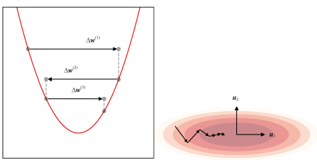
Momentum helps cross the valley faster

Nesterov momentum: An improved momentum method: first “pre-step” according to the historical momentum, then compute the gradient at that position.

• Corrects the direction more promptly, reducing overshoot.
• Has a faster theoretical convergence rate, and often outperforms standard momentum in practice.

Adaptive Learning Rate Algorithms

Intuition: The previous algorithms use the same learning rate for all parameters, but different parameters may need different step sizes — some parameters are already close to optimal and need small, slow steps; others are still far off and need large steps forward. The core idea of adaptive learning rate algorithms is to “teach students according to their aptitude” — automatically assigning an appropriate learning rate to each parameter.

AdaGrad

AdaGrad (Adaptive Gradient) maintains an independent accumulated squared gradient for each parameter:

For the $i$-th parameter $w_i$, an $r_i$ value is maintained, which records the sum of squares of all its historical gradients.

The learning rate is adjusted to:

where $\delta$ is a small constant to prevent division by zero.

• For parameters that are updated frequently (large gradients): $r_i$ grows fast, the learning rate $\frac{\eta}{\sqrt{r_i}}$ drops fast, and the update step becomes smaller.
• For parameters that are rarely updated (small gradients): $r_i$ grows slowly, the learning rate stays relatively large, and the update step is larger.

Disadvantage: $r_i$ keeps accumulating, causing the learning rate to decrease monotonically, and training nearly stalls in the later stages.

RMSProp

RMSProp (Root Mean Square Propagation) improves on AdaGrad by using an exponential moving average (Exponential Moving Average, an averaging method where recent data has greater weight and distant data is gradually “forgotten”) to compute the squared gradient:

where $\beta$ (decay rate, taking values in 0~1, usually taken as 0.9) controls the “forgetting” speed — the larger $\beta$ is, the more it relies on historical gradients; the smaller $\beta$ is, the more it values the current gradient.

Update formula:

• If a parameter keeps changing a lot (large gradient) → r is large → learning rate becomes smaller → update step becomes smaller
• If a parameter rarely changes (small gradient) → r is small → learning rate is larger → update step is larger It can “forget” early gradients, avoiding premature decay of the learning rate. It always remembers all the paths previously traveled, becoming more and more cautious, with smaller and smaller steps.

Adam

Intuition: Adam (Adaptive Moment Estimation) is like a “smart climber” — it both remembers the directions it has walked before (momentum / first moment) and observes the ups and downs of the terrain underfoot (adaptive learning rate / second moment), automatically adjusting the step size according to the road conditions. It is currently the most commonly used optimizer, virtually without equal.

Combining momentum and RMSProp, where $\beta_1$ and $\beta_2$ are the decay rates of the first and second moments respectively (usually $\beta_1 = 0.9$, $\beta_2 = 0.999$):

First moment (momentum — remembers the directional trend of the gradient): $\mathbf{s}^{(\tau)} = \beta_1 \mathbf{s}^{(\tau-1)} + (1 - \beta_1) \frac{\partial E(\mathbf{w})}{\partial \mathbf{w}}$

Second moment — remembers the magnitude variation of the gradient: $\mathbf{r}^{(\tau)} = \beta_2 \mathbf{r}^{(\tau-1)} + (1 - \beta_2)(\frac{\partial E(\mathbf{w})}{\partial \mathbf{w}})^2$

Bias correction: at the beginning, because initialization is zero, the first few estimates are not very accurate and need correction:

Final update formula:

• $\hat{\mathbf{s}}^{(\tau)}$: tells us which direction to go (momentum)
• $\sqrt{\hat{\mathbf{r}}^{(\tau)}}$: tells us how large a step each parameter should take (adaptive learning rate)

Normalization Techniques

Intuition: Imagine an assembly line where the parts (data) handled at each station (layer) vary greatly in size — some huge, some tiny, making it hard for the workers to handle. Batch normalization (Batch Normalization, standardizing the data of each mini-batch) is like adding a “standardization machine” in front of each station, unifying the part sizes into a reasonable range, so the workers (the network) can work efficiently.

Batch Normalization

Normalize each feature of each mini-batch (subtract the mean, divide by the standard deviation), then scale and shift using learnable parameters $\gamma, \beta$ (scale and shift parameters, letting the network itself decide the optimal data range).

Advantages:

• Reduces internal covariate shift (Internal Covariate Shift, the phenomenon where the input distribution of each layer of the network keeps changing during training).
• Allows a larger learning rate, accelerating convergence.
• Has a certain regularization effect.

Layer Normalization

Layer Normalization (Layer Normalization) normalizes a single sample across all its features, without depending on the batch, and is suitable for RNNs (Recurrent Neural Networks) and Transformers (an architecture based on the attention mechanism).

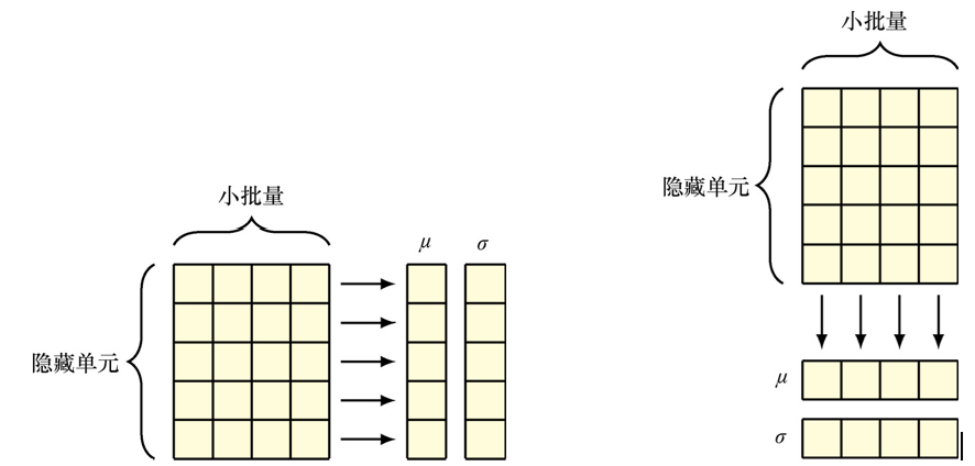
Left: batch normalization, right: layer normalization.

Chapter 7 Summary

One-sentence version: Gradient descent is “going down the mountain” — walking along the steepest direction; SGD is “sampling estimation” — looking at only a few points each time to decide the direction; momentum is “a ball rolling down a slope” — using inertia to rush through small pits; Adam is a “smart climber” — automatically adjusting the step size; normalization is a “standardized assembly line” — keeping data within a reasonable range.

Knowledge map:

1
Gradient descent optimization
2
├── Basis: error surface → gradient points uphill → go downhill in the opposite direction
3
├── Data strategy
4
│   ├── Batch gradient descent: use all data (slow but accurate)
5
│   ├── SGD: use a single sample (fast but noisy)
6
│   └── Mini-batch: compromise (most commonly used in practice)
7
├── Solve oscillation → Momentum (inertia acceleration)
8
├── Solve learning rate selection → Adaptive algorithms
9
│   ├── AdaGrad: accumulate squared gradient (decays to zero)
10
│   ├── RMSProp: exponential moving average (can "forget")
11
│   └── Adam: momentum + adaptive (default first choice)
12
├── Normalization techniques
13
│   ├── Batch normalization: standardize across samples
14
│   └── Layer normalization: standardize within a single sample
15
└── Parameter initialization → He initialization, symmetry breaking

Chapter 8 Backpropagation

Computing the Gradient

Intuition first: Imagine a factory assembly line where the final product has a quality problem. You need to trace responsibility — which worker (parameter) at which step caused the problem? Backpropagation (Backpropagation, an algorithm that efficiently computes each parameter’s contribution to the error in a neural network) starts from the final error and traces backward layer by layer along the network, computing how much “responsibility” each parameter should bear. Essentially, it is a systematic application of the chain rule (Chain Rule, the differentiation rule for composite functions).

Training a neural network typically involves minimizing an error function $E(\mathbf{w})$, where $\mathbf{w}$ represents all the weight and bias parameters of the network. The most commonly used method is gradient-based optimization algorithms (such as gradient descent), so efficiently and accurately computing the gradient $\nabla_{\mathbf{w}} E$ is crucial.

Forward Propagation and Backpropagation

The core idea of the backpropagation algorithm is to use a local message passing (Local Message Passing, where each node only needs to exchange information with adjacent nodes) scheme, passing the error information from the output end of the network backward to the input end.

1. Forward propagation (Forward Propagation, the process where data flows layer by layer from the input layer to the output layer):

   • Input data $\mathbf{x}_n$ passes through the network, computing the activation value $a_j$ (the weighted sum of inputs received by a neuron) and the output value $z_j$ (the final output after processing by the activation function) for each unit layer by layer.
   • For the $j$-th unit, its activation $a_j$ is the weighted sum of all its inputs $z_i$: $a_j = \sum_i w_{ji} z_i$.
   • Then apply the activation function $h(\cdot)$ (Activation Function, a function that introduces nonlinear transformation, such as sigmoid, ReLU, etc.) to obtain the output: $z_j = h(a_j)$.
   • Finally obtain the network output $\mathbf{y}$, and compute the error function $E$ (usually for a single data point $n$, denoted as $E_n$).

2. Backpropagation (Backward Propagation, the process where error information is passed backward layer by layer from the output layer):

   • Starting from the output layer, compute the “sensitivity” or “error term” $\delta_j$ of each unit to the error (i.e., the partial derivative of the error with respect to that unit’s activation, measuring how much “responsibility” that unit bears for the final error).
   • For an output unit $k$, $\delta_k$ is defined as the partial derivative (Partial Derivative, the derivative when only one variable changes and others are fixed) of the error function $E_n$ with respect to that unit’s activation $a_k$: $$\delta_k = \frac{\partial E_n}{\partial a_k}$$ For example, for the mean squared error $E_n = \frac{1}{2} \sum_k (y_k - t_k)^2$, we have $\delta_k = (y_k - t_k) h'(a_k)$.
   • For a hidden unit $j$, its error term is computed from the error terms of subsequent layers via the chain rule: $$\begin{align} \delta_j = \frac{\partial E_n}{\partial a_j} = \sum_k \frac{\partial E_n}{\partial a_k} \cdot \frac{\partial a_k}{\partial a_j}=\sum_k \frac{\partial E_n}{\partial a_k} \cdot \frac{\partial a_k}{\partial z_j} \cdot \frac{\partial z_j}{\partial a_j}\\ =\sum_k \frac{\partial E_n}{\partial a_k} \cdot w_{kj} \cdot h'(a_j) = h'(a_j) \sum_k w_{kj} \delta_k \end{align}$$ This formula shows that the error of a hidden unit is the sum of the products of all connection weights at its output end and the downstream error terms, multiplied by the derivative of its activation function.
     • $\sum_k w_{kj} \delta_k$: the “contribution” of unit $j$ to the final error equals the weighted sum of its influence on all lower-layer units
     • $w_{kj}$: the influence weight of unit $j$ on unit $k$
     • $\delta_k$: the sensitivity of unit $k$ to the error
     • product $w_{kj} \delta_k$: the error transmitted through the connection $j \rightarrow k$
     • $h'(a_j)$: the modulating effect of the activation function on error propagation
     • if the activation function changes gently at this point (small derivative), error propagation weakens; if the activation function changes sharply at this point (large derivative), error propagation strengthens

3. Gradient computation:

   • Once all the $\delta_j$ of all units are computed, the partial derivative of the error function $E_n$ with respect to any weight $w_{ji}$ can be directly computed: $$\frac{\partial E_n}{\partial w_{ji}} = \delta_j z_i$$ This result is very concise: the gradient equals the error term $\delta_j$ at the output end of the target weight multiplied by the activation value $z_i$ at its input end.

The backpropagation algorithm can be summarized in the following steps (for a single data point $n$):

1. Forward propagation: compute the activation $a_j$ and output $z_j$ of all units.
2. Compute output errors: for each output unit $k$, compute $\delta_k = \partial E_n / \partial a_k$.
3. Backpropagate errors: from back to front layer by layer, for each hidden unit $j$, compute $\delta_j = h'(a_j) \sum_k w_{kj} \delta_k$.
4. Compute gradients: for each weight $w_{ji}$, compute $\partial E_n / \partial w_{ji} = \delta_j z_i$.

For batch or mini-batch training, the gradient of the total error $E$ is the sum of the gradients of all data points in the batch:

A Simple Example

To illustrate the backpropagation algorithm concretely, consider a standard two-layer feedforward network (one hidden layer, one output layer), using the sum-of-squares error function.

Network structure and notation:

• Input layer: $D$ input units $x_i$ ($i=0, 1, ..., D-1$), where $x_0 = 1$ is the bias term.
• Hidden layer: $M$ hidden units $z_j$ ($j=1, 2, ..., M$).
• Output layer: $K$ output units $y_k$ ($k=1, 2, ..., K$).

Use superscripts $(1)$ and $(2)$ to distinguish the weights of the two layers:

• $w_{ji}^{(1)}$: the weight from input unit $i$ to hidden unit $j$. (superscript 1 = layer 1, subscript ji = from i to j)
• $w_{kj}^{(2)}$: the weight from hidden unit $j$ to output unit $k$. (superscript 2 = layer 2, subscript kj = from j to k)

Tip for reading notation: the subscript is always “where it comes from → where it goes”, and the superscript is “which layer”. For example, $w_{kj}^{(2)}$ means “in layer 2, the weight from j to k”.

Forward Propagation Computation

For a training sample $n$:

1. Compute the weighted input of the hidden layer: $$a_j = \sum_{i=0}^{D-1} w_{ji}^{(1)} x_i \quad (j=1,...,M)$$
2. Compute the activation output of the hidden layer: Using the hyperbolic tangent (tanh) as the activation function: $$z_j = \tanh(a_j)$$ Its derivative has a simple form: $z_j' = 1 - z_j^2$.
3. Compute the weighted input of the output layer: $$a_k = \sum_{j=0}^{M} w_{kj}^{(2)} z_j \quad (k=1,...,K)$$ (Note: $z_0 = 1$ is the bias of the hidden layer)
4. Compute the activation output of the output layer: Using the linear activation function (i.e., the identity function): $$y_k = a_k$$ Its derivative is 1.
5. Compute the error: Using the sum-of-squares error: $$E_n = \frac{1}{2} \sum_{k=1}^K (y_k - t_k)^2$$

Backpropagation Computation (Computing Gradients)

1. Compute the error term $\delta_k$ of the output layer: Since the output layer activation function is linear, $h'(a_k) = 1$. $$\delta_k = (y_k - t_k) \cdot 1 = y_k - t_k \quad \text{see above for formula source}$$
2. Compute the error term $\delta_j$ of the hidden layer: According to the backpropagation formula: $$\delta_j = h'(a_j) \sum_k w_{kj}^{(2)} \delta_k$$ Substituting $h'(a_j) = 1 - \tanh^2(a_j) = 1 - z_j^2$: $$\delta_j = (1 - z_j^2) \sum_{k=1}^K w_{kj}^{(2)} \delta_k$$
3. Compute weight gradients:

• Gradient of the second-layer weight $w_{kj}^{(2)}$:

  $$\frac{\partial E_n}{\partial w_{kj}^{(2)}} = \delta_k \cdot z_j$$

• Gradient of the first-layer weight $w_{ji}^{(1)}$:

  $$\frac{\partial E_n}{\partial w_{ji}^{(1)}} = \delta_j \cdot x_i$$

• Complexity:

  • The computation of one forward propagation is roughly $O(W)$, where $W$ is the total number of weights in the network.
  • The computation of one backpropagation is also roughly $O(W)$.
  • Therefore, the total cost of computing all $W$ gradients is $O(W)$.

Thus, backpropagation provides a computationally feasible method for training large neural networks.

Jacobian Matrix

Hessian Matrix

Automatic Differentiation

Backpropagation is a special case of automatic differentiation (Automatic Differentiation, a technique for precisely computing the gradient of any differentiable function in a computer program, more powerful and efficient than symbolic and numerical differentiation). It is more powerful and efficient than symbolic differentiation (deriving formulas) and numerical differentiation (approximate computation).

Core Idea

The key idea of automatic differentiation is to decompose the computation process of a function into a series of basic, differentiable elementary operations (such as addition, subtraction, multiplication, division, exponentiation, logarithm, trigonometric functions, etc.). By tracking the execution of these basic operations (usually represented as a computation graph (Computation Graph, a directed graph using nodes and edges to represent computation steps and their dependencies) or computation trace), and applying the chain rule, it automatically builds the code for computing gradients.

Automatic differentiation has two main modes: (the book has two examples on P213 for better understanding)

1. Forward mode:

   • While computing the function value, compute its derivative with respect to some input variable.
   • It introduces an extra “tangent” variable $\dot{z}_i$ for each intermediate variable $z_i$ (called the “primal variable”), representing that variable’s derivative with respect to some input.
   • During forward propagation, compute the tuple $(z_i, \dot{z}_i)$ simultaneously.
   • For a function with $D$ inputs, computing the full gradient requires $D$ forward-mode computations.

2. Reverse mode:

   • The mode used by backpropagation.
   • First perform one forward propagation, compute and store the values $z_i$ of all intermediate variables.
   • Then perform one backpropagation, introducing an “adjoint” variable $\bar{z}_i$ for each intermediate variable $z_i$, representing the partial derivative of the final output with respect to $z_i$.
   • Starting from the output, using the stored intermediate values, compute each $\bar{z}_i$ backward according to the chain rule.
   • For a function with $K$ outputs and $D$ inputs, computing the Jacobian matrix from all outputs to all inputs, the reverse mode is usually more efficient than the forward mode, especially when $K << D$ (which is exactly the case for neural networks, where $K$ is the scalar error and $D$ is the massive number of parameters).

Relationship with Backpropagation

Backpropagation is the concrete implementation of reverse-mode automatic differentiation applied to the neural network error function. It efficiently computes the gradient $\nabla_{\mathbf{w}} E$ of the scalar error $E$ with respect to all network parameters $\mathbf{w}$.

The core of modern deep learning frameworks (such as PyTorch, TensorFlow) is a reverse-mode automatic differentiation engine. Users only need to write the forward propagation code (defining the network and loss function), and the framework automatically computes the gradient, without manually deriving complex partial derivative formulas.

Chapter 8 Summary

One-sentence version: Backpropagation = systematic application of the chain rule. Starting from the output error, trace “responsibility” backward layer by layer, compute the gradient of each parameter; the computation cost is about the same as one forward propagation.

Knowledge map:

1
Backpropagation
2
├── Forward propagation: data → compute activations layer by layer → output → compute error
3
├── Backpropagation: error → compute error term δ layer by layer → obtain gradient
4
│   ├── Output layer: δ = (prediction - truth) × activation function derivative
5
│   └── Hidden layer: δ = activation function derivative × weighted sum of downstream δ
6
├── Gradient formula: ∂E/∂wⱼᵢ = δⱼ × zᵢ (concise!)
7
├── Complexity: O(W), same as forward propagation
8
└── Extended applications
9
    ├── Jacobian matrix: sensitivity of output to input
10
    ├── Hessian matrix: curvature of the error surface
11
    └── Automatic differentiation: framework computes the gradient for you automatically

Chapter 9 Regularization

Intuition first: Remember the example of fitting data with a high-degree polynomial from Part 1? (see Chapter 1 - Regularization Term) When the polynomial degree is too high, the curve wildly wiggles to pass through every training point — this is overfitting (Overfitting, the phenomenon where a model performs very well on training data but poorly on new data). Regularization (Regularization, a family of techniques that prevent overfitting by constraining model complexity) is like putting a “tightening curse” on the model — preventing it from wiggling around too freely, so it learns smoother, more generalizable patterns.

How to improve the model’s generalization ability on limited training data by introducing inductive bias (Inductive Bias, a learning algorithm’s preference for a certain hypothesis)

Earlier (in Chapter 1 - Regularization Term) we saw regularization used to solve the overfitting problem in polynomial curve fitting. Its core idea is: add a penalty term to the loss function to limit the magnitude of the model parameters.

The form of the regularized error function is:

where:

• $E(\mathbf{w})$ is the original error function (e.g., mean squared error)
• $\mathbf{w}$ is the model parameter vector
• $\Omega(\mathbf{w})$ is the regularization term (the part that penalizes model complexity, e.g., $\frac{1}{2} \mathbf{w}^T\mathbf{w}$)
• $\lambda$ is the regularization hyperparameter (Regularization Hyperparameter, the “knob” controlling the regularization strength — the larger it is, the heavier the penalty and the simpler the model)

Regularization essentially introduces a certain bias in the bias-variance tradeoff (Bias-Variance Tradeoff, where higher model complexity means lower bias but higher variance, and vice versa) to significantly reduce the model’s variance, thereby improving generalization performance.

Inductive Bias

Most machine learning tasks are inverse problems (Inverse Problem, a problem of inferring causes from limited results): we only have limited sample data, yet we must infer the entire data distribution. Since there are infinitely many possible distributions that could generate this data, a preference must be introduced to select a specific solution. This preference is called inductive bias or prior knowledge (Prior Knowledge, the assumption held before seeing the data).

For example:

• Assume small changes in the input lead to small changes in the output → encourage the model to learn smooth functions
• In image recognition, the position of an object does not affect its category → introduce translation invariance

Without inductive bias, learning from data is impossible. Learning is essentially using prior knowledge to narrow down the hypothesis space.

“No Free Lunch” Theorem

On all possible problems, the average performance of all learning algorithms is the same. If some algorithm performs better on certain problems, it must perform worse on others.

• Deep neural networks are powerful because they have built-in inductive biases suited to real-world problems (such as smoothness, locality)
• The “general-purpose learning algorithm” we pursue is actually about finding inductive biases applicable to broad practical scenarios
• For specific tasks, adding stronger domain-specific biases yields better results

Symmetry and Invariance

Many tasks require the model output to remain invariant under certain transformations of the input. For example:

• Translation invariance: changing the object’s position in an image does not change the classification result
• Scale invariance: changing the object’s size does not change the classification result

Learning these invariances from data alone is very difficult, because a tiny translation may cause drastic changes in pixel values, and the combinations of transformations grow exponentially.

Four methods to achieve invariance:

1. Preprocessing: extract features invariant to the transformation (e.g., SIFT)
2. Regularized error function: penalize the change of the output under input transformations (e.g., tangent propagation)
3. Data augmentation: add transformed samples during training (e.g., flipping, rotating images)
4. Network structure design: embed the invariance into the network structure (e.g., convolutional neural networks)

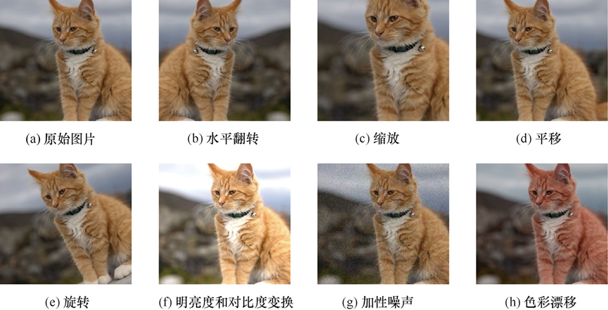
Data augmentation example

The introduction of the above inductive biases will be reflected concretely in later chapters: the regularization term reflects a preference for parameters, the network structure design reflects a preference for function form, and data augmentation reflects a preference for transformation invariance.

Weight Decay

Generalized Weight Decay

The general form of simple quadratic regularization:

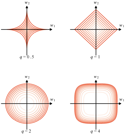
Regularization function contour lines for different q values

Generalized regularization using $q=1$ is called L1 regularization (also called Lasso, which uses the sum of absolute values of weights as the penalty term):

Its characteristic is: produces sparse solutions (Sparse Solution, i.e., many weights are pushed exactly to zero), achieving automatic feature selection (the weights corresponding to unimportant features directly become zero, as if “eliminated”).

Basic Form

The most common regularization term is the sum of squared weights (L2 regularization, also called Ridge or weight decay, which uses the sum of squares of weights as the penalty term):

The corresponding regularized error function is:

In gradient descent, its gradient is:

This means that after each update, the weights “decay” a bit (multiplied by $(1 - \eta\lambda)$), hence the name “weight decay”.

Regularization “suppresses” parameters that have little influence on the error, driving them toward zero. The number of parameters that actually take effect is called the effective number of parameters. As $\lambda$ increases, the effective number of parameters decreases.

Consistent Regularizer

Standard weight decay treats all weights equally, but when a linear transformation (such as normalization) is applied to the input or output, the optimal weights transform accordingly. Standard regularization breaks this consistency, leading to models with different performance under different data preprocessing methods.

Layer-wise Regularization

Use different regularization coefficients for the weights of different layers, and exclude the bias term b:

where $W_1, W_2$ represent the weights of the first and second layers respectively.

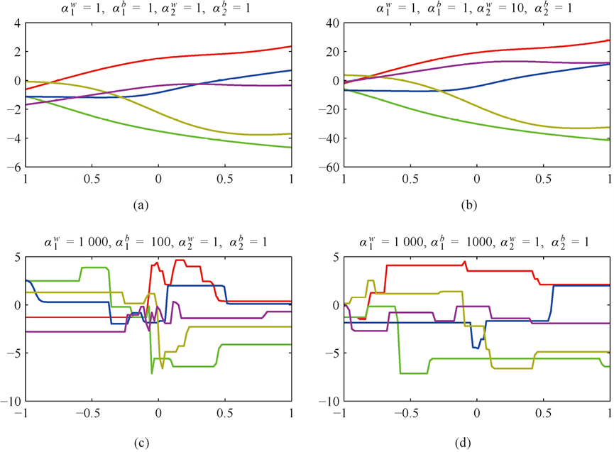
Layer-wise regularization

$a_1^w, a_1^b, a_2^w, a_2^b$ represent the first-layer bias, weights, and the second-layer bias, weights respectively.

Learning Curves

The learning curve (Learning Curve, a chart showing how the training and validation set errors change with the number of iterations during training) is an important tool for diagnosing the training state:

• Observe the training progress of the model;
• Determine whether overfitting has occurred;
• Control the effective complexity of the model.

In a typical training process, the training error usually decreases monotonically as the number of iterations increases. However, the validation set’s (Validation Set, a dataset not involved in training, specifically used to check the model’s generalization ability) error may first decrease and then rise, indicating that the model is starting to overfit the training data.

Early Stopping

Early stopping (Early Stopping, a technique that stops training when the validation set error no longer decreases) is an important technique for controlling the effective complexity of the model, and is widely used especially in deep learning. Its basic idea is:

Stop training when the validation set error reaches its minimum, rather than waiting until the training error fully converges.

• At the very beginning of training, the model complexity is low (e.g., weights are close to initial values, such as zero).
• As training proceeds, the model gradually fits the training data, the weights are continuously updated, and the model’s “effective complexity” gradually increases.
• If training continues, the model will overfit the training data, causing the validation error to rise.

Therefore, early stopping is equivalent to limiting the model’s effective number of parameters or effective complexity, thereby preventing overfitting.

For a quadratic error function, early stopping has an effect similar to L2 regularization (i.e., weight decay):

• Assume the weights start from the origin and update along the negative gradient direction.
• Due to the large differences in the eigenvalues of the Hessian matrix, the weight path will first descend rapidly along the low-curvature direction, then slowly approach the global minimum.
• If we stop at some intermediate point, the resulting weight vector ŵ is similar to that obtained using L2 regularization.

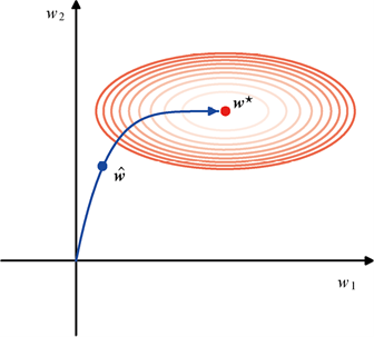
Early stopping and L2

$w^*$ represents the maximum likelihood solution corresponding to the minimum of the unregularized error function. If the weight vector starts from the origin and moves according to the local negative gradient direction, then the weight vector will advance along the path shown in the figure. By stopping training early, we can find a weight vector $\hat{w}$ closer to the origin. This is functionally similar to L2 adding the $\frac{\lambda}{2} \mathbf{w}^T\mathbf{w}$ term to the loss function, which biases the optimal solution toward the origin.

It can be proved mathematically that the product of the number of iterations and the learning rate, τη, in early stopping plays a role similar to the reciprocal of the regularization coefficient λ.

Double Descent

Double descent (Double Descent, a modern phenomenon: the test error first decreases, then rises, then decreases again in a non-monotonic behavior) breaks the traditional understanding of the bias-variance tradeoff:

• Training error decreases monotonically as complexity increases;
• Test error first decreases, then rises (the classic overfitting region), then decreases again

When the model complexity is large enough to completely fit the training data (i.e., training error is zero), the test error instead continues to decrease, and the model performs better.

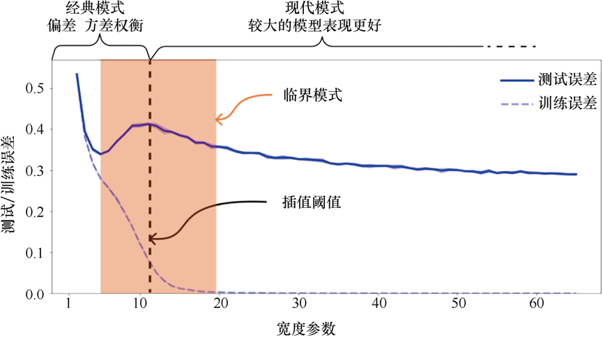
ResNet18 double descent

• Interpolation threshold: the minimum complexity required for the model to perfectly fit the training data.
• After the model complexity exceeds this threshold, it enters the “interpolation region”, where although the training error is zero, the test error may continue to decrease.

In the “critical complexity” region (i.e., near the peak of the test error), increasing the amount of training data may instead cause the test error to rise. Because more data pushes the “interpolation threshold” to the right, temporarily placing the model in a region more prone to overfitting.

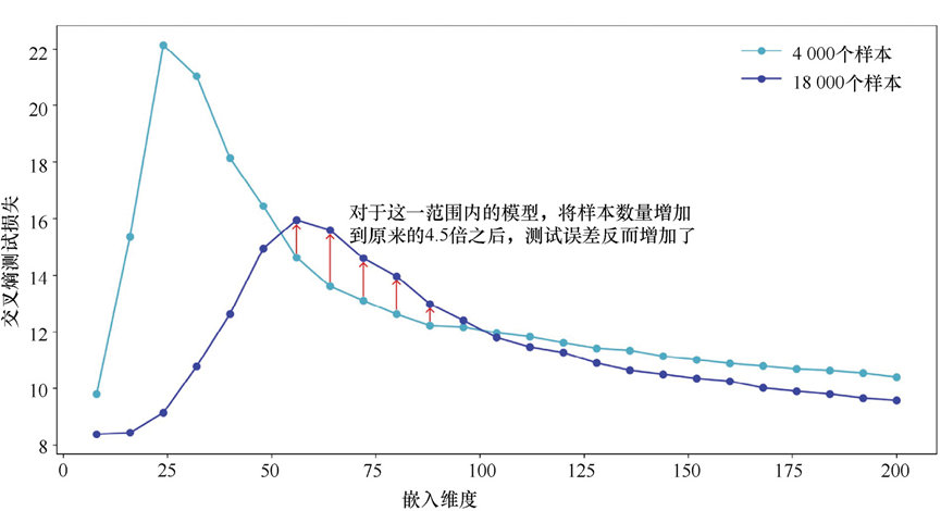
Transformer: increasing training data instead causes test error to rise

Significance:

1. Do not stop training too early: traditional early stopping may miss the later performance improvement
2. Long training may be beneficial: it makes sense that modern large models train for weeks or even months
3. Monitor the long-term changes in validation error: observe whether the double descent phenomenon appears

Parameter Sharing

Parameter sharing (Parameter Sharing, a technique that forces multiple locations in the network to use the same set of weights) is a hard constraint that forces a group of weights in the network to be set to the same value. These shared parameters are learned as a whole from the data.

• Advantage: significantly reduces the degrees of freedom of the model (i.e., the effective number of parameters), thereby lowering the risk of overfitting.
• Disadvantage: can only be used for specific problems, and requires knowing in advance which parameters should be shared.

Typical application: the convolution kernels in convolutional neural networks (CNNs). The same convolution kernel slides over the entire input image, its weights shared across all positions, embodying the prior knowledge of “translation invariance”.

Soft Parameter Sharing

Unlike hard sharing, soft sharing uses a regularization term to encourage a group of weights to tend toward similar values, rather than forcing them to be equal. This method is more flexible, and the “grouping” of shared weights can also be learned automatically during training.

Implementation:

• Use a Gaussian mixture model as the prior distribution of the weights: $$p(w) = \prod_i \left( \sum_{j=1}^K \pi_j \mathcal{N}(w_i | \mu_j, \sigma_j^2) \right)$$ where $K$ is the number of Gaussian components, and $\mu_j, \sigma_j, \pi_j$ are learnable parameters.
• The corresponding regularization term is the negative log prior: $$\Omega(w) = -\sum_i \ln \left( \sum_{j=1}^K \pi_j \mathcal{N}(w_i | \mu_j, \sigma_j^2) \right)$$
• The total error function is: $$E(w) = \tilde{E}(w) + \lambda \Omega(w)$$

Training mechanism:

• Introduce the posterior probability $\gamma_j(w_i)$: representing the probability that weight $w_i$ belongs to the $j$-th Gaussian component (computed via Bayes’ theorem).
• During gradient updates, each weight $w_i$ is pulled toward the mean $\mu_j$ of its affiliated Gaussian, with the pull strength determined by $\gamma_j(w_i)$.
• At the same time, $\mu_j, \sigma_j, \pi_j$ are also updated according to the posterior probabilities of all weights.

Optimization method:

• Use the EM algorithm for alternating optimization:
  • E-step: compute the posterior probability $\gamma_j(w_i) = \frac{\pi_j \mathcal{N}(w_i | \mu_j, \sigma_j^2)}{\sum_{k=1}^K \pi_k \mathcal{N}(w_i | \mu_k, \sigma_k^2)}$
  • M-step: update the parameters $\mu_j, \sigma_j, \pi_j$

Benefit of soft sharing: no need to pre-specify the grouping; allows weights to form multiple “clusters”; more flexible and adaptive.

Residual Connections

Similar to parameter sharing, the residual connection (Residual Connection, also called skip connection, a structure that lets information skip intermediate layers and pass directly to deeper layers) can also be viewed as a form of structured parameter sharing, achieving cross-layer parameter “sharing” through identity mapping. For a deeper discussion of residual networks, refer to Part 6.

As the number of network layers increases, training becomes increasingly difficult, and even with batch normalization and proper initialization, the following may still occur:

• Gradient vanishing/exploding: in deep networks, gradients are hard to propagate effectively.
• Gradient shattering: the gradient of a deep network is extremely sensitive to the input, becoming “noisy” and non-smooth, destroying the stability of gradient descent.

Theoretically, a deeper network should at least be no worse than a shallow one, but in practice a deeper network’s performance actually degrades.

Example: learning math

• Traditional way: it is too hard to learn directly from first grade all the way to PhD math; intermediate steps easily lose information, and you may forget the fundamentals after learning the later material.
• Residual way: retain the fundamentals at every stage; PhD math = fundamentals + newly learned content, and the fundamentals are always present (via the shortcut connection). Therefore the network only needs to learn the “incremental” part, so that even if the newly learned content is zero, the fundamentals are not lost.

Residual Block

Standard layer: $z = F(x)$,

Input x → layer 1 → layer 2 → … → layer L → output z

Residual layer: $z = F(x) + x$; where $F(x)$ is a nonlinear transformation (e.g., several convolutions + BN + ReLU), the part the network learns. (The network learns the mapping from x to (z-x), i.e., learns the “residual”)

Key idea: the network no longer directly learns the output $z$, but learns the “residual” $F(x) = z - x$.

Advantages

1. Identity mapping is easy to achieve:

• If the optimal solution is close to the identity transformation ($z \approx x$), just train the weights of $F(x)$ close to zero.
• Whereas in a plain network, achieving identity mapping requires precisely tuning a large number of parameters.

2. Gradient propagation is more stable:

• The residual connection provides a “shortcut” that allows the gradient to be passed back directly, alleviating the gradient vanishing problem.

3. The error surface is smoother:

• Experimental visualizations show that residual connections make the loss function surface smoother and the optimization path more stable.

4. Implicit ensemble effect:

• Expanding the residual network reveals it is equivalent to a parallel combination of multiple paths (of different depths).
• This gives the network both the stability of a shallow network and the expressive power of a deep network.

Implementation

• Dimension matching: when the input $x$ and the output $F(x)$ have different dimensions, adjust the shortcut path via a learnable linear transformation $W$: $$z = F(x) + Wx$$
• Connection position: usually add the residual connection before the ReLU activation (i.e., add first, then activate)

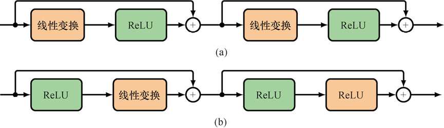
Two implementations of residual networks, combined as a residual block

Model Averaging

In machine learning, when we have multiple models to solve the same problem, rather than picking a single “best” model, averaging the prediction results of these models usually yields better generalization performance. This method of combining models is also called the committee method or ensemble method (Ensemble Method, a technique that combines the prediction results of multiple models to obtain better performance).

For models whose output is a probability distribution, the ensemble model’s prediction is the average of the individual models’ predictions:

• $p_l(y|x)$ is the output probability of the $l$-th model;
• $L$ is the total number of models.

This averaging operation helps reduce the variance in predictions, thereby improving overall performance.

From the perspective of the bias-variance decomposition, the prediction error of a single model can be decomposed into bias and variance:

When we average the predictions of multiple models, if these models’ errors are uncorrelated, then their variance components cancel each other out, reducing the overall error.

Imagine you are practicing dart throwing:

• Single model: you throw 10 times, all deviating from the bullseye but in similar ways → high bias, low variance
• Ensemble model: 10 people each throw 10 times; each person has their own bias (similar bias) but each person’s random errors differ (uncorrelated variance). Take each person’s average landing point, then average those 10 average points, and the result is closer to the center of the bullseye.

In practice we only have one dataset, so we need to artificially introduce differences between models. Common methods include:

1. Bootstrap aggregating:

• Randomly sample with replacement from the original dataset $X = \{x₁, ..., x_N\}$ to generate multiple new datasets of size $N$ (called bootstrap datasets).
• Each bootstrap dataset is used to train one model.
• The final prediction is the average of all models’ predictions.

2. Use models of different structures (e.g., different numbers of layers, different activation functions, etc.), then average.

Consider a regression problem with M trained models $y_1(x), ..., y_M(x)$, where the ensemble prediction is:

Let the true function be h(x), and each model’s output can be expressed as:

where $ε_m(x)$ is the $m$-th model’s error.

Average error of individual models:

Expected error of the ensemble model:

Assume the error mean is zero and the errors are uncorrelated

If the following hold:

• $E_x[ε_m(x)] = 0$
• $E_x[ε_m(x)ε_l(x)] = 0$ (when $m ≠ l$)

then we get:

It can be proved that the ensemble error will not exceed the average error of the individual models, i.e.: $E_{COM} ≤ E_{AV}$, so the ensemble is at least not worse.

Unlike bootstrap aggregating, boosting is a sequential ensemble method:

• Base classifiers are trained one by one;
• Each new classifier, when trained, pays more attention to the samples that previous classifiers got wrong (by increasing the weights of these samples);
• The final prediction combines the results of all base classifiers via weighted voting.

The advantage of boosting is that even if each base classifier is only slightly better than random guessing, the combination may still achieve very good performance.

Dropout

Intuition: Imagine a team where every day some people are randomly told to “take a day off” (not come to work). This way nobody can slack off expecting others to do their job, and everyone has to learn to complete tasks independently. Dropout (a technique that randomly “turns off” a portion of neurons during training) is exactly like this — each training session randomly lets some neurons “take a day off”, forcing every neuron to learn useful features, rather than relying on a few “star” neurons.

Dropout is a very effective regularization technique, which can be seen as implicitly performing approximate model averaging over an exponential number of sub-networks during training.

• In each training iteration, randomly “drop” (i.e., set to 0) a portion of neurons (including input and hidden layers, but not the output layer);
• Each time data is fed in, a new “mask” is generated, deciding which neurons are kept (typically the hidden layer keep probability ρ=0.5, the input layer ρ=0.8);
• Training only performs forward and backward propagation on the current “pruned” network.

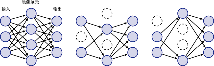
Dropout illustration (random ignore)

Effects:

1. Prevent co-adaptation:

• Each neuron cannot rely on the presence of other specific neurons;
• Must make useful contributions in many different contexts;
• Reduces overfitting to the noise in the training data.

2. Implicit model averaging:

• A network with M non-output nodes can theoretically generate $2^M$ different sub-networks;
• Dropout implicitly averages the predictions of these sub-networks during training.

Since it is infeasible to exactly average all $2^M$ sub-networks at test time (computationally intractable), there are two approximation methods:

1. Monte Carlo Dropout

• Keep dropout;
• Perform multiple forward propagations on the same input (each using a different dropout mask);
• Average the multiple outputs as the final prediction. $p(y|x) ≈ (1/T) * Σ_{t=1}^{T} p(y|x, R_t)$ where $R_t$ is the mask sampled at the t-th time.
• $T$ is typically 10-100 samples to obtain a stable result.

2. Weight scaling method (commonly used)

• Do not use dropout at test time;
• Multiply the trained weights by the keep probability ρ;
• This ensures the expected input to the neurons at test time is consistent with that during training.

Chapter 9 Summary

One-sentence version: Regularization = putting a “tightening curse” on the model, preventing it from overfitting too freely. L2 weight decay keeps weights from getting too large, early stopping keeps it from learning too long, Dropout keeps neurons from over-relying on teammates, and ensembling lets multiple models learn from each other’s strengths.

Knowledge map:

1
Regularization (prevent overfitting)
2
├── Why needed? → Inductive bias (prior knowledge narrows the hypothesis space)
3
├── Weight decay
4
│   ├── L2 (sum of squares): shrink weights overall, most common
5
│   ├── L1 (absolute value): produces sparse solutions, automatic feature selection
6
│   └── Layer-wise: different strengths for different layers
7
├── Training control
8
│   ├── Early stopping: stop when validation error no longer drops
9
│   └── Double descent: error drops again after crossing the interpolation threshold
10
├── Structural constraints
11
│   ├── Parameter sharing (hard sharing / soft sharing)
12
│   └── Residual connection (shortcut passes gradients)
13
└── Model averaging
14
    ├── Ensemble method: average multiple models
15
    └── Dropout: randomly turn off neurons during training

Cross-chapter connections: The regularization techniques in this part (L1/L2 weight decay) echo the penalty term for polynomial fitting in Part 1; for more details on residual connections, see Part 6.

Thanks for reading! Follow me if you'd like~

Deep Learning Notes - 4: Gradient Descent, Backpropagation, and Regularization

Mon Sep 01 2025

9029 words · 47 minutes

NotesDeep LearningLearningGradient DescentBackpropagationRegularization

---

© MuxiaoWF | CC BY-NC-SA 4.0

Share

Share this article

X (Twitter)TelegramRedditFacebookEmailQQ

Close

Close