Deep Learning Notes - 3: Classification Models and Introduction to Deep Neural Networks
Deep Learning Notes - 3, covering classification models (discriminant functions, logistic regression, softmax) and deep neural networks (activation functions, transfer learning, mixture density networks). Corresponding to Chapters 5-6 of "Deep Learning: Fundamentals and Concepts".
Part 3/8 of the series ← Previous | Next | Glossary
It is recommended to read Part 1 and Part 2 first. This part explains how to solve classification problems (from linear classifiers to neural networks), and why deep networks are stronger than shallow ones.
Chapter 5 Single-Layer Networks: Classification
In machine learning, the classification problem is one of the most fundamental and important tasks. This chapter introduces the basic principles of linear classification models, including core concepts such as discriminant functions, decision theory, generative classifiers, and discriminative classifiers.
Discriminant Functions
A discriminant function (a function that scores each class) defines a function for each class . For an input , it assigns it to the class with the highest discriminant function value:
Binary classification:
For a binary classification problem, we define the discriminant function . The decision boundary (the “dividing line” that separates different classes) is given by , which is a -dimensional hyperplane (a “plane” in high-dimensional space — a straight line in 2D space, an ordinary plane in 3D space, and a hyperplane in even higher dimensions).
To simplify the notation, we often introduce an extra “input” , and define the augmented weight vector and the augmented input vector , so that:
In this case, the decision boundary passes through the origin of the augmented input space.
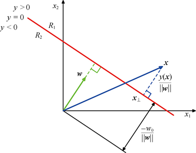
Binary classification
- Red line: represents the decision boundary , and divides the entire space into two regions: : the region where and : the region where
- Green vector : represents the weight vector (the normal vector of the decision boundary)
- Blue vector : represents the input sample
- Black vector : represents the projection of the input onto the decision boundary
- is the distance from the origin to the decision boundary (the offset of the decision boundary)
Multi-class:
- One-vs-rest classifier: train one classifier for each class , distinguishing from “not ”. This approach produces ambiguous regions, where some points are classified as positive by multiple classifiers or as negative by all classifiers.
- One-vs-one classifier: train a binary classifier for each pair of classes, requiring a total of classifiers. A new sample’s class is decided by majority voting. This approach also produces ambiguous regions.
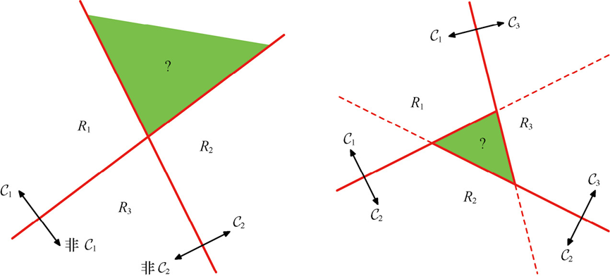
Multi-class (left: one-vs-rest classifier, right: one-vs-one classifier)
To avoid these problems, we adopt a single -class discriminant function consisting of linear functions:
Assign to the class that maximizes .
The decision boundary between classes and is defined by , that is:
This is a -dimensional hyperplane.
Properties of the decision regions: The decision region of such a -class linear discriminant function (i.e., the set of all points assigned to ) is simply connected and convex . This means that if any two points and within the region are connected, all points on the line segment between them also lie within the region.
In classification problems, the target variable is used to represent the class label.
- Binary classification: use binary encoding, . indicates class , and indicates class .
- Multi-class (): use 1-of-K encoding (also called one-hot encoding). The target vector is a vector of length , such that if the class is , then and the remaining elements are 0.
For example, for classes, the target vector for class 2 is:
We can interpret as the probability that the class is (the extreme case where the value is 0 or 1).
Decision Theory
Decision theory helps us make optimal classification decisions given the posterior probability (the probability that, after seeing the data , it belongs to a certain class), especially when different types of errors have different costs.
The loss matrix defines the cost incurred when a sample whose true class is is misclassified as .
where represents the cost of “true class is but predicted as ”. The diagonal entries are the cost of correct predictions (0), and the off-diagonal entries are the cost of making an error. is a “miss” (true predicted as false), and is a “false alarm” (false predicted as true). For example, in cancer screening: the cost of misclassifying a cancer patient () as healthy () (false negative) may be far higher than the cost of misclassifying a healthy person () as having cancer ( ) (false positive).
Minimizing Expected Loss
The optimal decision is to choose the class that minimizes the expected loss. For an input , the expected loss of classifying it as is:
We should choose the class that minimizes this expected loss.
For a two-class problem, this is equivalent to comparing the posterior probability against a threshold determined by the loss ratio.
Reject Option
Sometimes, when the classifier is uncertain about its prediction, it is better to choose to “reject” the classification and hand the sample over to a human or another, more complex system.
We can set a threshold , and if the maximum posterior probability is less than or equal to , the sample is rejected.
- : all samples are rejected.
- : no samples are rejected ( is the number of classes).
Adjusting controls the proportion of rejected samples.
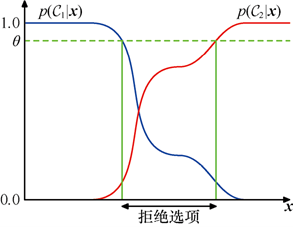
Reject option
This criterion can also be extended to the case where the reject decision itself has a cost (loss).
Inference and Decision
Solving a classification problem is usually divided into two stages:
- Inference stage: learn the model from the training data to obtain the posterior probability .
- Decision stage: use the posterior probability and decision theory (such as minimizing expected loss) to make the final class assignment.
Another approach is to directly learn a function from input to a decision, called a discriminant function. The linear discriminant functions discussed in this chapter belong to this approach.
Three ways to solve the decision problem (in decreasing order of complexity):
- Generative model: first model the class-conditional density (given the class, what the data looks like) and the prior probability (before seeing the data, the probability that each class occurs), then use Bayes’ theorem (deriving the probability of “cause → effect” from “effect → cause”) to compute the posterior . First understand what each class “looks like”, then judge which class a new sample most resembles based on its features. (A doctor diagnosing a disease first learns in detail the symptomatic characteristics of each disease, then looks at which symptoms the patient exhibits to determine the most likely disease.)
- Discriminative model: directly model the posterior probability . Directly learn how to distinguish between different classes, without caring what each class specifically “looks like” . (To distinguish apples from oranges, you only need to know that apples are redder and oranges are more orange; you do not need to know all the biological characteristics of apples and oranges in detail.)
- Direct mapping: directly learn a function from to a class label, such as the linear discriminant function in this chapter. Directly learn a decision rule without computing probabilities, outputting the class directly. (A simple rule: ” if an email contains ‘free’ it is spam”.)
Classifier Accuracy
The simplest performance measure is classification accuracy, i.e., the proportion of correctly classified test samples. However, when different errors have different costs, accuracy alone is insufficient.
Confusion Matrix
The confusion matrix provides a more detailed view of classification results. For a two-class problem, its form is as follows: (same as the loss matrix)
| Predicted: Healthy | Predicted: Cancer | |
|---|---|---|
| Actual: Healthy | ||
| Actual: Cancer |
- True Negative (TN): correctly predicted as healthy.
- False Positive (FP): incorrectly predicted as cancer (Type I error).
- False Negative (FN): incorrectly predicted as healthy (Type II error).
- True Positive (TP): correctly predicted as cancer.
ROC Curve
The ROC curve is a powerful tool for evaluating the performance of a binary classifier. It plots the True Positive Rate (TPR) against the False Positive Rate (FPR).
- Precision:
- True Positive Rate (TPR) = Recall:
- False Positive Rate (FPR):
- False Discovery Rate:
By changing the threshold of the classification decision, different points on the ROC curve can be obtained.
- Ideal classifier: the closer the point on the ROC curve is to the top-left corner, the better.
- Random classifier: the ROC curve is a diagonal line from the bottom-left to the top-right corner.
- Area Under the Curve (AUC): a single number that quantifies classifier performance. AUC = 0.5 indicates random guessing, and AUC = 1.0 indicates perfect classification.
The F-score is the harmonic mean of precision and recall, used to comprehensively evaluate classifier performance:
Exercise 1
In the validation set of a watermelon classification task, there are 10 examples in total, of which 3 examples are labeled “1”, indicating that the example is a good watermelon; and 7 examples are labeled “0”, indicating that the example is not a good watermelon. Due to limited learning ability, the method can only produce a classifier with accuracy 0.8 on the validation set.
- To obtain the best precision on the validation set, what prediction should the classifier make? What are the recall and F1 at this point?
An accuracy of 0.8 means 2 will be predicted incorrectly. To maximize precision , the incorrect predictions should be placed in FN, i.e., predict positive examples as negative. At this point recall ,
- To obtain the best recall on the validation set, what prediction should the classifier make? What are the precision and F1 at this point?
To maximize recall , the incorrect predictions should be placed in FP, i.e., predict negative examples as positive. At this point precision ,
Exercise 2
Suppose a dataset contains 8 examples, whose corresponding labels and the learner’s output values (sorted from largest to smallest) are shown in the table below. The task is a binary classification task, where a label of 1 or 0 indicates the true label being positive or negative. The learner’s output value represents the learner’s confidence that the example is positive (the probability that it considers the example to be positive).
| Example | X1 | X2 | X3 | X4 | X5 | X6 | X7 | X8 |
|---|---|---|---|---|---|---|---|---|
| Label | 1 | 1 | 0 | 1 | 0 | 1 | 0 | 0 |
| Learner output | 0.81 | 0.74 | 0.62 | 0.53 | 0.44 | 0.35 | 0.25 | 0.21 |
- Compute the coordinates of each endpoint on the P-R curve and plot it.
Predict each example as positive in descending order of output value
| ID | 1 | 2 | 3 | 4 | 5 | 6 | 7 | 8 |
|---|---|---|---|---|---|---|---|---|
| TP | 1 | 2 | 2 | 3 | 3 | 4 | 4 | 4 |
| FP | 0 | 0 | 1 | 1 | 2 | 2 | 3 | 4 |
| FN | 3 | 2 | 2 | 1 | 1 | 0 | 0 | 0 |
| TN | 4 | 4 | 3 | 3 | 2 | 2 | 1 | 0 |
| P | 1 | 1 | 0.666667 | 0.75 | 0.6 | 0.666667 | 0.571429 | 0.5 |
|---|---|---|---|---|---|---|---|---|
| R | 0.25 | 0.5 | 0.5 | 0.75 | 0.75 | 1 | 1 | 1 |
- Compute the coordinates of each endpoint on the ROC curve and plot it; compute the AUC (Area Under the ROC Curve).
| TPR | 0.25 | 0.5 | 0.5 | 0.75 | 0.75 | 1 | 1 | 1 |
|---|---|---|---|---|---|---|---|---|
| FPR | 0 | 0 | 0.25 | 0.25 | 0.5 | 0.5 | 0.75 | 1 |
AUC=0.5*0.25+0.75*0.25+1*0.5=0. 8125
Generative Classifiers
Generative classifiers follow the “generative model” path of decision theory (method 1 of “Inference and Decision” above): first model the data distribution (class-conditional density) of each class and the prior probability of the class, then use Bayes’ theorem to compute the posterior probability , and finally make a decision.
Continuous Inputs (Gaussian Class-Conditional Density)
Assume the input is continuous, and the data of each class follows a Gaussian distribution (the normal distribution — see Part 2). This is the most common case.
Class-conditional density: for class , we have
where is the mean vector (the “center” of the data), and is the covariance matrix (describing the “shape” and “orientation” of the data — the correlations between dimensions).
Prior probability: can be estimated from the training data, for example, , where is the number of samples in class , and is the total number of samples.
According to Bayes’ theorem, the posterior probability is:
where is the normalization constant.
To classify, we compare the posterior probabilities of different classes. Since the denominator is the same for all classes, we only need to compare the numerator . Equivalently, we can compare their logarithms:
This is called the evidence or activation. We assign to the class that maximizes .
For a two-class problem, we define the discriminant function:
If , assign to ; otherwise assign to . The decision boundary is given by .
Linear Discriminant Analysis (LDA) is an important special case that assumes all classes share the same covariance matrix (i.e., the data of each class has the same “shape” and “orientation”, only the “center position” differs): .
Under this assumption, substituting the Gaussian density expression into and performing the algebra, we find that the quadratic terms in cancel out.
Ultimately, the discriminant function becomes a linear function of :
where
Since the discriminant function is linear, the decision boundary is a hyperplane, hence the name “Linear Discriminant Analysis”.
Quadratic Discriminant Analysis: if we do not assume that all classes share the same covariance matrix, i.e., can differ, then in the expression for , the quadratic terms in will not cancel out.
In this case, the discriminant function is a quadratic function of , and the decision boundary is a quadratic surface (such as an ellipse, hyperbola, etc.).
Quadratic Discriminant Analysis is more flexible than Linear Discriminant Analysis, but it requires estimating more parameters, so it may overfit on small datasets.
Discrete Inputs
When the input is a discrete variable, a different class-conditional density model is needed.
A common example is the Naive Bayes classifier (“naive” because it makes a bold simplifying assumption), which assumes that, conditioned on class , the input features are conditionally independent (once the class is known, the value of one feature does not affect the value of another feature):
For binary inputs (), is usually modeled with a Bernoulli distribution.
Although the “naive” assumption (feature independence) rarely holds in reality, the Naive Bayes classifier often performs well in practice (such as in text classification).
Discriminative Classifiers
Discriminative classifiers follow the “discriminative model” path of decision theory (method 2 above): they directly model the posterior probability , rather than first modeling the class-conditional density.
Fixed Basis Functions
When the decision boundary of the data is not a straight line (or hyperplane), a linear model cannot handle it well. To model nonlinear decision boundaries, we can map the original input to a feature space composed of fixed nonlinear basis functions (pre-defined nonlinear transformation functions).
Lego bricks vs. custom parts: fixed basis functions are like a pre-built set of Lego bricks — you can only assemble using the existing blocks, whether or not they fit your data. The advantage is easy assembly; the disadvantage is that when you encounter a special shape, the bricks do not match. The neural networks discussed later are like a machine that can “cast parts” on the spot — its basis function parameters are learnable and can automatically adjust their shape according to the data.
Specifically, the original input data is mapped through some fixed nonlinear functions to a new feature space, where the originally complex nonlinear relationship may become linearly separable.
Then, we assume that the posterior probability is a nonlinear transformation of a linear function of these features.
Logistic Regression
Binary classification:
We directly assume that the posterior probability of class has the following form:
where is the logistic sigmoid function — which we will see frequently:
and is a linear function of (or a linear function in the feature space ):
Therefore,
The posterior probability of the other class is .
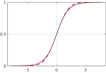
The S-shaped curve of the logistic sigmoid function (red), mapping a real number a to the (0,1) interval
Parameter learning: learn the weights through Maximum Likelihood Estimation (MLE, choosing the set of parameters that maximizes the probability of the observed data).
For the training set (where is 1-of-K encoding), the likelihood function is:
where .
Maximizing the likelihood is equivalent to minimizing the cross-entropy (a measure of the difference between two probability distributions — the smaller it is, the more accurate the prediction) error function:
This error function can be minimized by optimization algorithms such as gradient descent (updating parameters along the direction of fastest error decrease).
For classes, we use the softmax function (also called the normalized exponential function — it converts a set of arbitrary real numbers into a probability distribution, so that all outputs are positive and sum to 1; we will also see this frequently later) to convert the linear activations (the weighted input value of a certain neuron in the network) into posterior probabilities.
Define the activation of the -th class as:
Then the posterior probability is:
The softmax function ensures that all lie in the (0,1) interval and sum to 1.
Suppose we have activations for three classes:
Computation: , , , sum =
Softmax output: , ,
Parameter learning: again use maximum likelihood estimation.
For the target vector (1-of-K encoding), the likelihood is:
where is the -th element of .
This corresponds to minimizing the multi-class cross-entropy error:
where .
If the class-conditional density belongs to the exponential family distribution, and all classes share the same basis function , then the resulting posterior probability exactly has the form of softmax.
Probit Regression
Probit regression is another discriminative model, based on a “noisy threshold” model.
- Compute a linear activation .
- Assume there is a random threshold with probability density .
- If , predict ; otherwise predict .
Then, the probability of predicting is the probability that is greater than the random threshold , that is:
where is the cumulative distribution function (CDF) of — the cumulative probability from negative infinity to (see Part 2).
If is the standard normal distribution , then is called the probit function. It has a shape similar to the logistic sigmoid function, but with slightly different tails.
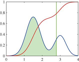
Reject option
On the left is the probability density of the threshold (blue), and on the right is its cumulative distribution function (red). The figure illustrates how is determined by the cumulative area of
Chapter 5 Summary
One-sentence version: The essence of the classification problem is to draw a line (or a surface) to separate data of different classes. How is this line drawn? It can be drawn directly (discriminant function), or by first understanding what each class of data looks like and then drawing (generative model), or by directly learning a probability (discriminative model). How well it is drawn is measured by metrics such as ROC and AUC.
Knowledge map:
Discriminant functions├── Binary classification: a linear function y = w^T x + w0, decision boundary is a hyperplane└── Multi-class: K linear functions, softmax / one-vs-rest / one-vs-one
Decision theory├── Loss matrix: different error types have different costs (e.g., misclassifying cancer vs normal)├── Minimize expected loss: choose the class that minimizes expected loss└── Reject option: hand to human when uncertain
Three classification approaches├── Generative model: first learn p(x|Ck) and p(Ck), then use Bayes' theorem│ ├── Linear Discriminant Analysis (LDA): shared covariance → linear boundary│ └── Quadratic Discriminant Analysis (QDA): different covariance → quadratic boundary├── Discriminative model: directly learn p(Ck|x)│ ├── Logistic regression (binary): sigmoid + cross-entropy│ └── softmax classifier (multi-class): softmax + multi-class cross-entropy└── Direct mapping: directly learn x → class label
Performance evaluation├── Confusion matrix: TP / FP / FN / TN├── ROC curve: TPR vs FPR, closer to top-left is better└── AUC / F-score: single number summarizing classifier performanceChapter 6 Deep Neural Networks
In the previous chapter, we learned about linear regression and classification models, which are usually based on a linear combination of fixed nonlinear basis functions of the input. For example, a classification model can be expressed as:
where is a pre-defined basis function (such as polynomial, Gaussian, etc.), and is the output activation function (such as the sigmoid function).
Such models are theoretically “universal approximators” — with enough suitable basis functions, they can approximate any nonlinear function. However, they face severe limitations in practice, especially in high-dimensional input spaces.
Limitations of Fixed Basis Functions
Curse of Dimensionality
When the number of input variables increases, the complexity of the fixed basis function approach rises sharply. This is not just a theoretical problem — it fundamentally limits the feasibility of fixed basis function methods on high-dimensional data.
- Polynomial regression: the number of parameters of a third-order polynomial in -dimensional space grows as . For high-dimensional data (such as images), this leads to an explosion in the number of parameters.
- Grid-based classifier: if we divide the input space into a regular grid, where each grid corresponds to a basis function, then the number of grids grows exponentially with dimension — each additional dimension doubles the number of grids. In a 10-dimensional space with just 10 bins per dimension, we would need (10 billion) bins, far exceeding the number of samples in any practical dataset.
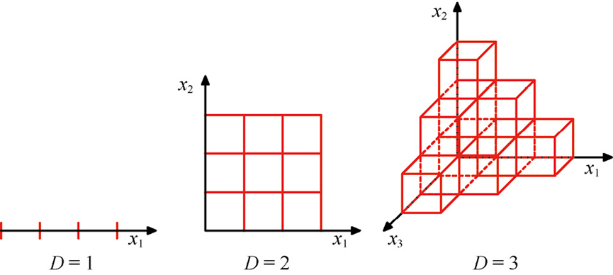
The growth trend of the number of small bins when divided into grids in 1D, 2D, and 3D spaces. In high-dimensional space, most grids are empty, causing the model to fail to classify new samples
This shows that if the basis functions are fixed in advance and uniformly distributed in the input space, then in high-dimensional cases they become extremely sparse and cannot effectively utilize the limited training data.
Our intuition in low-dimensional space often fails in high-dimensional space. For example:
- Volume distribution of a hypersphere: in high-dimensional space, the volume of a unit hypersphere is almost entirely concentrated in a thin shell near the surface. This means most points are “far from the center” — imagine a 100-dimensional ball where 99% of the volume is in a thin shell less than 1% of the radius from the surface.
- Probability mass of a Gaussian distribution: the probability mass of a multidimensional Gaussian distribution is also concentrated on a thin shell at a certain specific radius, rather than near the origin — this is completely different from the intuition in a 2D bell curve where “the closer to the center, the higher the probability”.
- “Emptiness” of high-dimensional space: in high-dimensional space, the distances between data points tend to become equal. The difference between the nearest neighbor and the farthest neighbor becomes negligible, and the concept of “distance” itself becomes meaningless.
Data Manifold
Data manifold: refers to the low-dimensional structure that high-dimensional data actually distributes on. Although the data may have thousands of dimensions (such as the pixels of an image), the truly meaningful variation may be only a few dimensions (such as the position and rotation angle of an object).
Real-world data (such as images and speech), although represented in high-dimensional space (e.g., a 64×64 pixel image has 4096 dimensions), actually only occupies a low-dimensional submanifold of the entire space.
For example:
- The variation of handwritten digit images is mainly controlled by a few factors such as position, rotation, and scaling, so these images are roughly distributed on a three-dimensional manifold.
- Randomly generated pixel images are completely different from real images because they lack the strong correlations in real data (the difference between two adjacent pixels is usually small).
Therefore, we do not need to define basis functions over the entire high-dimensional space, but only on the data manifold. This greatly reduces the number of required basis functions.
Data-Dependent Basis Functions
To solve the problem of fixed basis functions, we can make the basis functions depend on the training data itself.
Radial Basis Function Network (RBF): each training sample acts as the center of a basis function, with the form:
where is the -th training sample (the “center” of the basis function), and is the width parameter (controlling how wide this “hill” is — the larger is, the wider the influence range; the smaller is, the stronger the response is only near ). is the squared Euclidean distance from the input point to the center. Simply put: the closer to the training sample, the larger the output value.
This method can automatically adapt to the data distribution, but is computationally expensive and prone to overfitting.
Support Vector Machine (SVM): similarly uses data points as basis function centers, but reduces the number of effective basis functions by optimizing the selection of support vectors.
Although these methods are more flexible than fixed basis functions, they still cannot effectively handle large-scale datasets and are difficult to scale to complex tasks. This leads to deep neural networks — a model that can automatically learn multi-level representations.
Multi-Layer Neural Networks
The core idea of deep neural networks is: let the basis functions themselves also have learnable parameters, and jointly optimize all parameters through gradient descent.
Two-Layer Network Structure
A simple two-layer neural network contains:
First layer (hidden layer):
where is the nonlinear activation function (a function that performs a nonlinear transformation on the weighted sum result), and is called a hidden unit (a neuron in the middle layer of the network — neither input nor output, hence called “hidden”).
Second layer (output layer):
where is the output activation function (chosen according to the task, such as sigmoid, softmax).
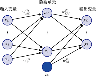
Two-layer network structure
Universal Approximation
Theory shows that, with enough hidden units, a two-layer neural network can approximate any continuous function to arbitrary precision. This shows that neural networks have powerful representational capacity.
However, universal approximation only guarantees “existence”, not that the learning algorithm can find the optimal solution, nor how many hidden units are needed. In practice, deep networks are often more efficient than shallow ones.
Hidden Unit Activation Functions
Hidden units must use nonlinear activation functions, otherwise the entire network is equivalent to a linear model (unable to capture nonlinear relationships).
Common activation functions include:
- Logistic Sigmoid: , compresses any real number into the interval. Commonly used early on, but when the absolute value of the input is large, the gradient approaches zero (vanishing gradient), making deep network training difficult.
- tanh: , output in , with mean close to zero, making training more stable. It can be understood as an “upgraded version” of sigmoid — the output is zero-centered and has better gradient properties.
- hard version: , a linear approximation of tanh, faster to compute.
- softplus: , the “smooth version” of ReLU — behaves similarly to ReLU, but is a smooth curve rather than a sharp corner near zero, and more computationally complex.
- ReLU (Rectified Linear Unit): , the mainstream choice for modern deep networks. Intuitively it is a “switch” — negative values are all turned off (output 0), and positive values pass through unchanged. Extremely simple to compute, and the gradient in the positive interval is always 1, completely avoiding vanishing gradients. (Preferred)
- leaky ReLU: , gives the negative interval a small slope (usually 0.01), avoiding ReLU’s “dead neuron” problem (some neurons always output 0 and can no longer be activated). (Choose when ReLU has problems)
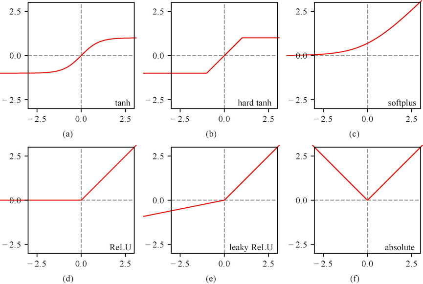
Various activation functions
Symmetry in Weight Space
In multi-layer neural networks, especially those with hidden layers, if we swap all the connection weights of two hidden units in the same hidden layer, the overall behavior of the network does not change.
For a two-layer network, if we swap the weights of hidden units and :
- (weights from input to hidden layer)
- (weights from hidden layer to output)
The output of the network remains unchanged, because this is equivalent to relabeling the hidden units.
Weights of hidden unit 1: [0.5, 0.3]; weights of hidden unit 2: [0.2, 0.7]
Swap all connections of these two hidden units: weights of hidden unit 1: [0.2, 0.7] (originally unit 2’s) weights of hidden unit 2: [0.5, 0.3] (originally unit 1’s)
The final output of the network is completely unchanged
For neural networks using symmetric activation functions (such as tanh), if we flip the signs of all input and output weights of a certain hidden unit at the same time:
While keeping the bias unchanged, the output of the network also does not change, because the symmetric activation function satisfies .
For a network using the tanh activation function:
Originally: the weight is +0.5, the input is +2, compute tanh(0.5 × 2) = tanh(1)
After flipping: the weight is -0.5, the input is -2, compute tanh((-0.
Due to the property tanh(-x) = -tanh(x), the final result is the same
Deep Networks
Although a two-layer network is a universal approximator, deep networks (multiple hidden layers) have significant advantages:
- Hierarchical representation: shallow layers learn low-level features such as edges and textures, while deep layers learn high-level features such as semantics and objects.
- Parameter efficiency: for some complex functions, deep networks can achieve them with fewer parameters, while shallow networks may require an exponential number of hidden units.
- Generalization ability: deep structures can better capture the intrinsic hierarchical structure of data, improving performance on complex tasks (such as image recognition and natural language processing).
An -layer deep network can be formally expressed as:
where , is the input, is the output, is the activation function of the -th layer, and is the weight and bias parameter matrix.
Representation Learning
Representation learning means: letting the machine automatically learn effective representations of the input data, rather than relying on hand-designed features.
Early on, training deep networks was very difficult. A key breakthrough was unsupervised pre-training (without using labeled data, let the network learn the structure of the data by itself).
- Pre-training stage: use unsupervised learning layer by layer (such as autoencoders or restricted Boltzmann machines) to initialize the network weights. Each layer first learns how to reconstruct its input, thereby discovering the intrinsic structure of the data.
- Fine-tuning stage: connect the entire network and use labeled data and gradient descent for supervised fine-tuning.
This method provides the network with good initial weights through pre-training, making it easier to converge.
Important progress: later research found that under suitable conditions (such as using ReLU activation functions, appropriate weight initialization, batch normalization, etc.), the pre-training stage can be skipped entirely, and deep networks can be trained end-to-end (from raw input directly to final output, without manually designed intermediate steps) using supervised learning starting from random initialization. This simplifies the process and makes deep learning more accessible.
However, the ideas of pre-training and representation learning remain crucial, especially in data-scarce domains. The most famous example is the Transformer model (such as BERT, GPT) in natural language processing. These models are first pre-trained on massive unlabeled text (for example, by predicting masked words or the next word) to learn a deep internal representation of language. Afterwards, this pre-trained model can be used for various downstream tasks (such as question answering, translation), achieving excellent performance through fine-tuning.
Transfer Learning
Transfer learning is a technique that uses knowledge learned on one task to improve the performance of another related task. It is particularly suitable for situations where the labeled data of the target task (Task A) is scarce. Its core idea is:
A network trained on a large-scale dataset (Task B) has already learned general, low-level features of the input data (such as images) (e.g., edges, textures, basic shapes). These features are useful for many vision tasks. Transfer learning exploits these already-learned feature representations.
- Source task training: first train a deep network on a data-rich, related task (such as classification of everyday objects on ImageNet). The early layers of this network learn general image features.
- Target task application:
- Feature extractor: use the early layers (usually the convolutional layers) of the pre-trained network as a fixed feature extractor. Pass the new data of the target task through this fixed network to obtain a high-level feature representation.
- Classifier training: on these extracted features, train a new, simple classifier (usually the last few layers of the network) to solve the target task (such as skin lesion classification).
- Fine-tuning: if the target task has enough data, the entire network (or only the last few layers) can be further fine-tuned to adapt to the specific features of the new task. Fine-tuning usually uses a very small learning rate to prevent destroying the useful knowledge already learned in the pre-trained model.
Advantages:
- Improved accuracy: compared to training from scratch, transfer learning usually achieves higher accuracy because it exploits the general knowledge learned from large amounts of data.
- Save time and resources: avoids the large amount of computational resources and time required to train a large network from scratch.
- Alleviate data scarcity: makes it possible to train effective models in domains with very few labeled data.
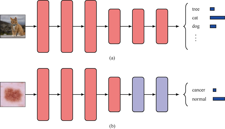 (a) The network is trained on a large-scale dataset (such as ImageNet);
(b) Copy the weights of the early layers (red) as a fixed feature extractor, and retrain the last few layers (blue) to adapt to the new task (such as skin lesion classification).
Contrastive Learning
Contrastive learning is a self-supervised learning (no manual labeling required, constructing the learning signal from the data itself) paradigm aimed at learning good data representations without large amounts of labeled data.
Its core idea is: pull similar samples (positive pairs) closer in the representation space, while pushing dissimilar samples (negative pairs) farther apart.
- Instance discrimination: treat different augmented versions of the same image (such as rotation, cropping) as positive pairs, and different images as negative pairs.
- Supervised contrastive learning: treat different images of the same class as positive pairs.
- Cross-modal contrastive learning (such as CLIP): treat an image and its corresponding text description as a positive pair.
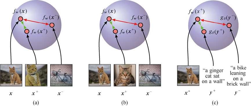
(a) Instance discrimination (b) Supervised contrastive learning (c) CLIP model
General Network Architectures
In addition to standard fully-connected feedforward networks, more complex architectures can be designed.
- Residual Network (ResNet): introduces skip connections (allowing the signal to “skip” intermediate layers and pass directly to later ones), allowing information to bypass certain layers and propagate directly. This helps alleviate the vanishing gradient problem in deep networks (the gradient decays layer by layer during backpropagation in deep networks, causing the earlier layers to barely learn), making it possible to train very deep networks.
- Graph Neural Network: handles graph-structured data, where both nodes and edges have features.
The key requirement is that the network must be feedforward (acyclic), to ensure that the output is a deterministic function of the input.
Tensors
In deep learning, data, weights, and activations are usually represented in the form of tensors (a general term for multi-dimensional arrays — a scalar is a 0th-order tensor, a vector is 1st-order, a matrix is 2nd-order, and higher dimensions are collectively called tensors).
- Scalar: 0-dimensional tensor (a single number).
- Vector: 1-dimensional tensor (an array of numbers).
- Matrix: 2-dimensional tensor (a table of numbers).
- Tensor: higher-dimensional arrays.
For example, a dataset containing color images can be represented as a 4D tensor: , where is the height, is the width, and is the number of channels (RGB is 3).
Tensors are the foundation of modern deep learning frameworks (such as PyTorch, TensorFlow), and GPUs are very good at tensor operations.
Error Functions
Summary subsection — corresponding to Section 6.4 of the original book
Choosing an appropriate error function is crucial for training neural networks. The error function is usually the negative log-likelihood (turning “maximize the probability of the data occurring” into “minimize the error” — see the discussion of maximum likelihood in Part 1 and Part 2).
Regression
Prerequisite: Chapter 2 - Maximum Likelihood and Least Squares
For regression tasks, the target variable is real-valued. Assume the target value follows a Gaussian distribution with the network output as the mean (see Part 2 - Gaussian Distribution):
where is the output of the neural network, and is the noise variance.
At this point, the activation function of the output unit uses the identity function (i.e., linear output): .
Given an independent and identically distributed training dataset , the corresponding likelihood function is:
The corresponding negative log-likelihood error function is:
which is equivalent to minimizing the sum-of-squares error function:
Minimizing this error function is equivalent to maximizing the likelihood function (the probability of the data given the parameters — see Part 1 and Part 2). Due to the nonlinearity of the network, this error function is usually non-convex, making it difficult to find the global optimum.
When there are multiple target variables, assuming they are independent and share the noise variance given the input and parameters, the conditional distribution is:
The corresponding error function is:
The noise variance can be estimated by:
where is the dimension of the target variable.
Binary Classification
Prerequisite: Logistic Regression Chapter 2 - Bernoulli Distribution
For binary classification tasks, the target variable , indicating membership in class or .
The network uses one output unit, with the logistic sigmoid function as the activation function:
At this point can be interpreted as the posterior probability , and as .
The conditional distribution of the target variable follows the Bernoulli distribution:
The corresponding negative log-likelihood error function is the cross-entropy error function:
Research shows that, compared to the sum-of-squares error, the cross-entropy error leads to faster training speed and better generalization performance.
If independent binary classification tasks need to be performed, output units can be used, each with a sigmoid activation function, and the total error is the sum of the cross-entropies of each output:
Multi-class Classification
Prerequisite: Discriminative Classifier - Multi-class
For a -class classification problem, each sample belongs to one and only one class. Using 1-of-K encoding, only one element in the target vector is 1 and the rest are 0.
The network uses output units, with the Softmax function as the activation function:
Softmax ensures the output satisfies and , and can be interpreted as the posterior probability .
The corresponding error function is the multi-class cross-entropy error function:
The combination of Softmax and multi-class cross-entropy is the standard choice for multi-class classification problems.
One-sentence version:
- Regression task: linear output + sum-of-squares error
- Binary classification task: Sigmoid output + binary cross-entropy error
- Multi-class classification task: Softmax output + multi-class cross-entropy error
This pairing originates from the maximum likelihood estimation framework, ensuring consistency between the error function and the output distribution assumption. This principle is universal and can be extended to other conditional distribution forms.
Mixture Density Networks
A Mixture Density Network (MDN) is a more advanced model for handling cases where the output is a multimodal function of the input (the same input may correspond to multiple reasonable outputs). Its core idea is: predict multiple possible futures, rather than a single answer.
Problem Background
A standard regression network learns the conditional mean from input to output . This works well when the conditional distribution is unimodal (only one peak, i.e., only one “reasonable answer”). But when the distribution is multimodal (multiple peaks, i.e., multiple “reasonable answers”), the mean may lie between the two peaks — a “void zone” where no possible result would ever occur.
Multiple possible futures: imagine you are driving to an intersection and can turn left or right. If you let the model predict only one “average direction”, it will tell you to “go straight” — but there may be a wall there. The MDN’s approach is to tell you at the same time “70% chance of turning left, 30% chance of turning right”, so you can see all reasonable options.
For example, controlling a robot arm — the same end position may correspond to two different joint angles (elbow up or down). The average of these two solutions is not a valid joint configuration.
Mixture Density Network (MDN)
The MDN uses a mixture model (usually a Gaussian mixture model) to model the conditional probability density :
where:
- is the mixture coefficient of the -th Gaussian component (i.e., what proportion of the whole this component occupies), satisfying and .
- is the mean of the -th Gaussian.
- is the variance of the -th Gaussian.
The output layer of the network has units, outputting , , and respectively ( is guaranteed to be positive).
The MDN is trained by maximizing the log-likelihood of the data. The error function is:
Prediction
The MDN can output the entire conditional distribution, not just a point estimate. We can:
- Predict the conditional mean: .
- Predict the conditional variance: , which depends on .
- Predict the conditional mode (the most likely value): usually take the mean of the Gaussian component with the largest mixture coefficient.
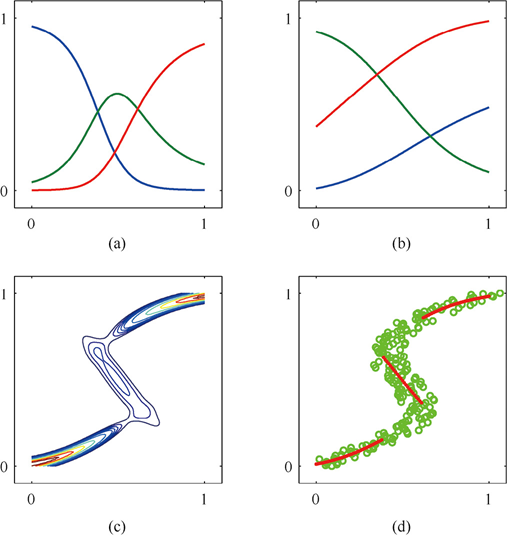
MDN
(a) Mixture coefficients
The three colors represent the mixture coefficients of three different Gaussian components. At different positions of the input , the contribution weight of each Gaussian component to the overall distribution. For example: when is small, is larger, indicating the first Gaussian component dominates; when is close to the middle value, peaks, indicating the second component plays the main role; when is large, dominates.
This shows that the MDN can dynamically adjust the importance of each component according to the input.
(b) Means
The three colors represent the means of three different Gaussian components, showing the trend of the center position of each Gaussian component as the input changes. Together they define the “modes” of the conditional distribution (i.e., the possible output values). For example: in some regions, and correspond to two different output paths respectively; while lies between them, possibly used for smooth transitions or filling gaps.
(c) Conditional probability density contour plot
(d) Conditional mode
Green circles: represent the true training data points Red curve: represents the conditional mode predicted by the MDN (i.e., the most likely output value), obtained by selecting the mean of the Gaussian component with the largest mixture coefficient.
Chapter 6 Summary
One-sentence version: Fixed basis functions “explode” in high-dimensional space (curse of dimensionality), so we need to let the basis functions learn by themselves — this is the core idea of neural networks. Deep networks are stronger than shallow ones in “hierarchical understanding”; transfer learning and contrastive learning let the model reuse already-learned knowledge, and the MDN can handle scenarios where “one input corresponds to multiple reasonable outputs”.
Knowledge map:
Limitations of fixed basis functions├── Curse of dimensionality: number of parameters grows exponentially with dimension, data becomes sparse├── Data manifold: real data actually only occupies a low-dimensional substructure of high-dimensional space└── Data-dependent basis functions: RBF / SVM, use training data to define basis function centers
Multi-layer neural networks├── Structure: input → hidden layer (learnable basis functions) → output layer├── Activation functions: ReLU (preferred) / sigmoid / tanh / softplus├── Universal approximation: a two-layer network can theoretically approximate any continuous function└── Weight symmetry: swapping hidden units does not change the output
Deep networks├── Hierarchical representation: shallow layers learn edges/textures, deep layers learn semantic objects├── Representation learning: from hand-crafted features to automatically learned features├── Transfer learning: large model pre-training → fine-tuning on small data└── Contrastive learning: pull similar samples closer, push dissimilar samples apart
Error function pairings├── Regression: linear output + sum-of-squares error├── Binary classification: sigmoid + cross-entropy└── Multi-class classification: softmax + multi-class cross-entropy
Mixture Density Network (MDN)└── Use Gaussian mixture model to model p(t|x), output the entire distribution rather than a single prediction