Part 2/8 of the series ← Previous | Next | Glossary

It is recommended to read Part 1 first (foundations of probability theory). This part covers common probability distributions, the probabilistic derivation of linear regression, and the bias-variance tradeoff.

Chapter 3 Standard Distributions

This chapter assumes that all observed data are independent and identically distributed

Discrete Variables

Bernoulli Distribution

Intuition: Flipping a coin, the outcome is either heads (1) or tails (0), and the probability of heads is $\mu$. The Bernoulli distribution is the mathematical description of this “black or white” scenario—it characterizes the probability of a single binary random variable (a binary random variable, one that can only take the value 0 or 1) $x \in \{0, 1\}$. Its probability mass function (the probability description of a discrete variable) is:

where $\mu$ is the probability that $x=1$, with $0 \leq \mu \leq 1$. The expectation and variance of this distribution are respectively:

Given an independent and identically distributed (i.i.d., each sample is unaffected by the others and comes from the same distribution) dataset $\mathcal{D} = \{x_1, ..., x_N\}$, its likelihood function (a measure of how well the parameters explain the data) is:

The log-likelihood function is:

By maximizing the log-likelihood (taking the derivative with respect to the parameter and setting it to zero), we obtain the maximum likelihood estimate (Maximum Likelihood, ML, the parameter value that maximizes the probability of the data occurring):

also known as the sample mean; here $m$ is the number of observations in the dataset for which $x=1$. This shows that the maximum likelihood estimate is simply the proportion of “success” events in the sample.

Binomial Distribution

Intuition: A coin is flipped $N$ times; what is the probability that heads comes up exactly $m$ times? This is the question answered by the Binomial distribution—it describes the probability of the total number of “successes” $m$ in $N$ independent Bernoulli trials (each an independent coin flip). Its probability mass function is:

The expectation and variance of this distribution are:

As $N \to \infty$, by the central limit theorem, the binomial distribution approaches the Gaussian distribution (normal distribution).

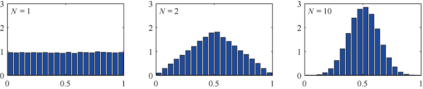
As N increases, the binomial distribution approaches the Gaussian distribution (normal distribution)

Multinomial Distribution

Intuition: Rolling a die, the six faces each have different probabilities of coming up. If you roll it $N$ times, how many times does each face appear? The Multinomial distribution is the generalization of the Bernoulli distribution from “flipping a coin” to “rolling a die”—it handles the case of multiple categories ($K$ states). Consider a $K$-state discrete variable (a variable that can only take a finite number of values) $x$, represented using 1-of-$K$ encoding (only one of $K$ positions is 1, the rest are 0, also called one-hot encoding) as $x = (x_1, ..., x_K)^T$. Let $\mu_k$ be the probability that $x_k=1$, satisfying $\sum_{k=1}^K \mu_k = 1$. For a single observation, its distribution is:

For $N$ independent observations, let $m_k$ be the number of times the $k$-th state appears (i.e., $m_k = \sum_{n=1}^N x_{nk}$); then the multinomial distribution is (proof omitted):

Its maximum likelihood estimate is:

Multivariate Gaussian Distribution (Normal Distribution)

Univariate Gaussian Distribution

Let us recall the univariate (one-dimensional) normal distribution mentioned earlier:

The probability density function of the univariate Gaussian distribution (normal distribution) is:

where $\mu$ is the mean, $\sigma^2$ is the variance, $\sigma$ is the standard deviation, and $\beta = 1/\sigma^2$ is the precision. The latter part of the expression can be understood as normalization.

Multivariate Gaussian Distribution

Intuition: Imagine a cloud in the shape of an ellipsoid, with data points densely clustered near the center and becoming sparser toward the outside. The Multivariate Gaussian distribution (also called the multivariate normal distribution) is the mathematical description of this “dense in the middle, sparse around the edges” ellipsoidal distribution. For a $D$-dimensional random vector (a vector composed of multiple random variables) $\mathbf{x}$, the multivariate Gaussian distribution is:

(which can be understood as the cumulative result of the one-dimensional case) where $\mathbf{\mu}$ is the $D$-dimensional mean vector (a vector composed of the average values along each dimension), and $\mathbf{\Sigma}$ is the $D \times D$ covariance matrix (a symmetric positive-definite matrix that describes the spread of each dimension and the correlations between dimensions). $\mathbf{\Sigma}^{-1}$ is called the precision matrix (the inverse of the covariance matrix). The latter part of the expression can similarly be understood as normalization.

For the two-dimensional case, the covariance matrix is written out as:

$$\mathbf{\Sigma} = \begin{pmatrix} \text{var}(x_1) & \text{cov}(x_1, x_2) \\ \text{cov}(x_2, x_1) & \text{var}(x_2)\end{pmatrix}$$

The diagonal contains the variance of each dimension itself (its covariance with itself), and the off-diagonal contains the covariance between different dimensions (the tendency of $x_1$ and $x_2$ to vary together). Since the covariance matrix is symmetric, $\text{cov}(x_1, x_2) = \text{cov}(x_2, x_1)$.

Gaussian Geometry:

The equiprobability density surface (the surface formed by points of equal probability density) of the Gaussian distribution is determined by the quadratic form $\Delta^2 = (\mathbf{x} - \mathbf{\mu})^T \mathbf{\Sigma}^{-1} (\mathbf{x} - \mathbf{\mu})$, a quantity called the Mahalanobis distance (a “distance” measure that accounts for differences in scale across dimensions and correlations). When the covariance matrix $\mathbf{\Sigma}$ is the identity matrix, the Mahalanobis distance reduces to the ordinary Euclidean distance.

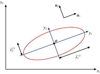
How the eigenvalues and eigenvectors of the covariance matrix affect the shape of the distribution (such as the direction and length of the principal axes of the ellipse)

The eigenvectors (vectors whose direction is unchanged under the matrix transformation) and eigenvalues (the corresponding scaling factors) of the covariance matrix $\mathbf{\Sigma}$ determine the shape of the Gaussian distribution. The eigenvectors define the directions of the principal axes, and the square roots of the eigenvalues are proportional to the lengths of the principal axes. (Proof omitted)

Moments

Intuition: If you imagine a probability distribution as a thin plate of irregular shape, then the “moments” are the statistics that describe the characteristics of this plate in different directions. The first moment is the center of gravity of the plate, and the second moment describes how “fat or thin” the plate is around its center of gravity. Specifically:

Conclusion: The first moment (expectation) equals the parameter $\mathbf{\mu}$, i.e., the “center of gravity” of the distribution. Mathematically:

Conclusion: The second moment is $E[\mathbf{xx}^T] = \mathbf{\mu}\mathbf{\mu}^T + \mathbf{\Sigma}$.

Covariance matrix:

When defining variance, we usually first subtract the mean—just as when measuring “how far from the center of gravity.” For the multivariate case, the covariance of the random vector $\mathbf{x}$ is defined as:

Substituting $E[\mathbf{x}] = \mathbf{\mu}$ and $E[\mathbf{xx}^T] = \mathbf{\mu}\mathbf{\mu}^T + \mathbf{\Sigma}$:

where $E[\mathbf{xx}^T]$ is the second moment and $E[\mathbf{x}]E[\mathbf{x}]^T$ is the square of the first moment.

Therefore, the parameter matrix $\mathbf{\Sigma}$ is precisely the covariance matrix of this Gaussian distribution, which determines the spread of the data in each direction and the correlation between variables.

Conditional and Marginal Gaussian Distributions

Intuition: Imagine a two-dimensional ellipsoidal cloud of data. If you “cut a slice” along a vertical line, the cross-section is still a one-dimensional Gaussian (bell curve); if you “project away” one of the dimensions, what remains is still a Gaussian. This is the closure property of the Gaussian distribution.

An important property of the Gaussian distribution is that both its conditional distribution (the distribution of the remaining variables given part of the variables) and its marginal distribution (the distribution of the remaining variables after ignoring some variables) are also Gaussian distributions.

Split $\mathbf{x}$ into two parts $\mathbf{x}_a$ and $\mathbf{x}_b$, and correspondingly partition the mean $\mathbf{\mu}$ and the covariance matrix $\mathbf{\Sigma}$:

• Conditional distribution: (split)

  $$p(\mathbf{x}_a|\mathbf{x}_b) = \mathcal{N}(\mathbf{x}_a|\mathbf{\mu}_{a|b}, \mathbf{\Sigma}_{a|b})$$

  where: (proof omitted)

  $$\mathbf{\mu}_{a|b} = \mathbf{\mu}_a + \mathbf{\Sigma}_{ab} \mathbf{\Sigma}_{bb}^{-1} (\mathbf{x}_b - \mathbf{\mu}_b), \quad \mathbf{\Sigma}_{a|b} = \mathbf{\Sigma}_{aa} - \mathbf{\Sigma}_{ab} \mathbf{\Sigma}_{bb}^{-1} \mathbf{\Sigma}_{ba}$$

  Note that the mean of the conditional distribution is a linear function of $\mathbf{x}_b$, and the covariance is independent of $\mathbf{x}_b$.

  
  

  In the proof, the block matrix inversion formula is used; it is included here as well:

  $$\begin{pmatrix} A & B \\ C & D \end{pmatrix}^{-1} = \begin{pmatrix} M & -MBD^{-1} \\ -D^{-1}CM & D^{-1} + D^{-1}CMBD^{-1} \end{pmatrix}$$

  where it is defined that:

  $$M = (A - BD^{-1}C)^{-1}$$

  The quantity $M^{-1}$ is called the Schur complement of the left matrix with respect to the submatrix $D$.

Suppose we have a two-dimensional Gaussian distribution: $\mathbf{x} = \begin{pmatrix} x_1 \\ x_2 \end{pmatrix} \sim \mathcal{N}\left(\begin{pmatrix} 0 \\ 0 \end{pmatrix}, \begin{pmatrix} 1 & 0.5 \\ 0.5 & 1 \end{pmatrix}\right)$ Now given $x_2 = 1$, find the conditional distribution of $x_1$:

$\mathbf{\mu}_a = 0$, $\mathbf{\mu}_b = 0$ $\mathbf{\Sigma}{ab} = 0.5$, $\mathbf{\Sigma}{bb} = 1$ $\mathbf{x}_b = 1$

Conditional mean:

Conditional variance:

So: $p(x_1|x_2=1) = \mathcal{N}(x_1|0.5, 0.75)$

• Marginal distribution: (dimensionality reduction, looking only at the probability distribution of $\mathbf{x}_a$) $$p(\mathbf{x}_a) = \mathcal{N}(\mathbf{x}_a|\mathbf{\mu}_a, \mathbf{\Sigma}_{aa})$$ If $\mathbf{x} \sim \mathcal{N}(\mathbf{\mu}, \mathbf{\Sigma})$, where: $$\mathbf{\mu} = \begin{pmatrix} \mu_1 \\ \mu_2 \\ \mu_3 \\ \mu_4 \end{pmatrix}, \quad \mathbf{\Sigma} = \begin{pmatrix} \sigma_{11} & \sigma_{12} & \sigma_{13} & \sigma_{14} \\ \sigma_{21} & \sigma_{22} & \sigma_{23} & \sigma_{24} \\ \sigma_{31} & \sigma_{32} & \sigma_{33} & \sigma_{34} \\ \sigma_{41} & \sigma_{42} & \sigma_{43} & \sigma_{44} \end{pmatrix}$$ then the marginal distribution of $\mathbf{x}_a = \begin{pmatrix} x_1 \\ x_2 \end{pmatrix}$ is: $$p(\mathbf{x}_a) = \mathcal{N}(\mathbf{x}_a|\mathbf{\mu}a, \mathbf{\Sigma}{aa})$$ where: $\mathbf{\mu}_a = \begin{pmatrix} \mu_1 \\ \mu_2 \end{pmatrix}$ $\mathbf{\Sigma}{aa} = \begin{pmatrix} \sigma_{11} & \sigma_{12} \\ \sigma_{21} & \sigma_{22} \end{pmatrix}$

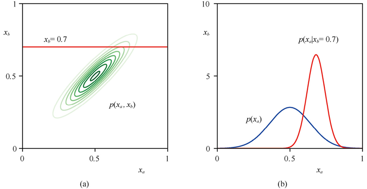
• The left figure shows the probability density function (PDF) of a two-dimensional Gaussian distribution, represented as contour lines. The contours are elliptical (see Gaussian Geometry above), centered at the mean point $(\mu_a, \mu_b) = (0.5, 0.5)$, and the direction of the principal axes of the ellipse is determined by the covariance matrix (there is positive correlation here because $\Sigma_{ab} > 0$). The denser the ellipse, the higher the probability density; the outer ellipses represent low-probability regions. The distribution has positive correlation ($x_a$ and $x_b$ vary in the same direction), manifested as the ellipse being stretched along the diagonal.

  The red horizontal line indicates the slice at $x_b = 0.7$, used to extract the conditional distribution.

• The right figure shows a one-dimensional distribution curve:

  The blue curve: $p(x_a)$ is the marginal distribution of $x_a$ (i.e., ignoring the influence of $x_b$).

  The red curve: $p(x_a|x_b=0.7)$ is the conditional distribution of $x_a$ given $x_b = 0.7$.

  The conditional distribution uses the observed value of $x_b$ to provide a more precise prediction of $x_a$.

  The marginal distribution only reflects the overall statistical properties of $x_a$ and does not depend on a specific value of $x_b$.

It can also be seen that: the conditional distribution of a Gaussian distribution is still a Gaussian distribution, and its mean and variance can be computed from the covariance matrix.

Bayes’ Theorem + Gaussian Distribution

Why read this section? This conclusion will be used repeatedly later—Bayesian linear regression, Gaussian processes, and probabilistic PCA all rely on it. To put it simply: if both the prior and the likelihood are Gaussian, then the posterior is also Gaussian—which is very convenient computationally, because a Gaussian distribution is completely described by just its mean and covariance.

When the prior distribution of one variable (see Part 1 - Bayes’ Theorem) and the conditional distribution of another variable are both Gaussian, the posterior distribution (the updated belief about the parameters after observing the data) is also a Gaussian distribution.

Consider two random variables $\mathbf{x}$ and $\mathbf{y}$. We have the following two distributions:

1. Prior distribution (the belief about the parameters before observing the data): $p(\mathbf{x}) = \mathcal{N}(\mathbf{x} | \mathbf{\mu}, \mathbf{\Lambda}^{-1})$

• This is the initial belief about $\mathbf{x}$, a Gaussian distribution with mean $\mathbf{\mu}$ and covariance matrix $\mathbf{\Lambda}^{-1}$ ($\mathbf{\Lambda}$ is the precision matrix).

2. Likelihood distribution (the probability of the observed data given the parameters): $p(\mathbf{y}|\mathbf{x}) = \mathcal{N}(\mathbf{y} | \mathbf{A}\mathbf{x} + \mathbf{b}, \mathbf{L}^{-1})$

• The probability of observing $\mathbf{y}$ given $\mathbf{x}$. It is also a Gaussian distribution, whose mean is the linear function $\mathbf{A}\mathbf{x} + \mathbf{b}$ of $\mathbf{x}$, with covariance matrix $\mathbf{L}^{-1}$.

Our goal is to use Bayes’ theorem to compute the posterior distribution $p(\mathbf{x}|\mathbf{y})$, i.e., the updated belief about $\mathbf{x}$ after observing $\mathbf{y}$.

Bayes’ theorem states:

First, we construct the joint distribution of $\mathbf{z} = (\mathbf{x}^T, \mathbf{y}^T)^T$ as $p(\mathbf{z}) = p(\mathbf{x}, \mathbf{y})$. By the definition of conditional probability:

Substituting the expressions for the two Gaussian distributions and taking the logarithm, we obtain the log form of the joint distribution:

After expanding and reorganizing, it can be found that $\ln p(\mathbf{z})$ is a quadratic form in $\mathbf{z}$. This shows that the joint distribution $p(\mathbf{z})$ itself is also a multivariate Gaussian distribution.

For a multivariate Gaussian distribution, its precision matrix (i.e., the inverse of the covariance matrix) can be obtained from the quadratic coefficient in the log probability density function. (The quadratic term $-\frac{1}{2} (\mathbf{x} - \mathbf{\mu})^T \mathbf{\Sigma}^{-1} (\mathbf{x} - \mathbf{\mu})$)

Extracting the quadratic term in $\mathbf{z}$ from the above expression, we obtain the precision matrix $\mathbf{R}$ of the joint distribution:

Using the block matrix inversion formula (see above, block matrix inversion), we can find the covariance matrix $\text{cov}[\mathbf{z}] = \mathbf{R}^{-1}$:

The expectation of $\mathbf{z}$ is:

1. Marginal distribution $p(\mathbf{y})$:

• Extracting the part of $\mathbf{y}$ from the mean and covariance of the joint distribution above: $$p(\mathbf{y}) = \mathcal{N}(\mathbf{y} | \mathbf{A}\mathbf{\mu} + \mathbf{b}, \mathbf{L}^{-1} + \mathbf{A}\mathbf{\Lambda}^{-1}\mathbf{A}^T)$$
• This shows that the mean of $\mathbf{y}$ is the result of the mean of $\mathbf{x}$ after linear transformation, and its covariance is the sum of the observation noise covariance ($\mathbf{L}^{-1}$) and the covariance introduced by the uncertainty of $\mathbf{x}$ ($\mathbf{\Lambda}^{-1}$) through the linear transformation.

2. Conditional distribution $p(\mathbf{x}|\mathbf{y})$:

• Using the properties of the block precision matrix (see above, block matrix inversion), we can directly write out the mean and covariance of $p(\mathbf{x}|\mathbf{y})$: $$p(\mathbf{x}|\mathbf{y}) = \mathcal{N}(\mathbf{x} | \mathbf{\Sigma} \{ \mathbf{A}^T \mathbf{L} (\mathbf{y} - \mathbf{b}) + \mathbf{\Lambda} \mathbf{\mu} \}, \mathbf{\Sigma})$$ where $$\mathbf{\Sigma} = (\mathbf{\Lambda} + \mathbf{A}^T \mathbf{L} \mathbf{A})^{-1}$$

Therefore:

• The posterior covariance $\mathbf{\Sigma}$ is jointly determined by the prior precision ($\mathbf{\Lambda}$) and the likelihood precision ($\mathbf{A}^T \mathbf{L} \mathbf{A}$), reflecting the combination of prior information and observed information.
• The posterior mean is a weighted average of the prior mean and the “prediction” based on the observation $\mathbf{y}$, with weights determined by their respective uncertainties (covariances).

Maximum Likelihood Estimation

Consider an independent and identically distributed dataset $\mathcal{D} = \{\mathbf{x}_1, ..., \mathbf{x}_N\}$, assumed to be generated by a multivariate Gaussian distribution $\mathcal{N}(\mathbf{x}|\mathbf{\mu}, \mathbf{\Sigma})$. Its log-likelihood function is:

Taking the derivative with respect to the mean $\mathbf{\mu}$ and the covariance matrix $\mathbf{\Sigma}$ respectively and setting the derivatives to zero yields the maximum likelihood estimates:

$\mathbf{\mu}_{\mathrm{ML}}$ is the sample mean, and $\mathbf{\Sigma}_{\mathrm{ML}}$ is the sample covariance. Similar to the univariate case, $\mathbf{\Sigma}_{\mathrm{ML}}$ is a biased estimate of the true covariance.

Sequential Estimation

Intuition: Imagine you are wearing a wristband while running that calculates your average pace. Every kilometer you run, the wristband corrects the previous estimate with the new data, rather than recalculating from scratch. Sequential estimation is this kind of online algorithm that “updates as it collects data.”

When data arrives in a streaming fashion (streaming, the data does not all arrive at once, but arrives one by one or in batches), a method is needed to update the parameter estimates online (without recomputing everything). For the mean, we can use:

This shows that the new estimate equals the old estimate plus a “correction term,” which is $1/N$ times the difference between the new data point and the old estimate; therefore, as $\mathbf{\mu}_N$ grows larger and larger, the contribution of later terms becomes smaller and smaller.

Gaussian Mixture Model

Intuition: If the data clearly has multiple “clusters” (for example, male and female heights each form a peak), fitting with a single Gaussian distribution is like trying to cover two peaks with just one bell curve—no matter how you cover it, it won’t fit. The idea of the Gaussian Mixture Model (GMM) is to superimpose multiple bell curves—one Gaussian per “cluster,” mixed together in proportion.

Although the Gaussian distribution has good analytical properties, a single Gaussian distribution (with only one peak) cannot capture complex data structures, such as multimodal (multiple peaks) data.

The Gaussian Mixture Model (GMM) solves this problem by linearly combining $K$ Gaussian distributions (summing multiple Gaussian distributions weighted by proportions):

where $\pi_k$ is the mixing coefficient of the $k$-th Gaussian component, satisfying $0 \leq \pi_k \leq 1$ and $\sum_{k=1}^K \pi_k = 1$. Each $\mathcal{N}(\mathbf{x}|\mathbf{\mu}_k, \mathbf{\Sigma}_k)$ is called a component.

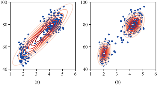
Left: unmixed Gaussian distribution fit; right: mixed Gaussian distribution fit (two peaks)

• By adjusting the number of components $K$, the mean $\mathbf{\mu}_k$, the covariance $\mathbf{\Sigma}_k$, and the mixing coefficient $\pi_k$ of each component, the Gaussian mixture model can approximate any continuous probability density function.
• For ease of analysis, a $K$-dimensional latent variable $\mathbf{z}$ (to distinguish multiple different groups) can be introduced, using 1-of-K encoding (see Chapter 5 - 1-of-K encoding) where only one element is 1 and the rest are 0. The position of the element that is 1 indicates which category the sample belongs to. $z_k=1$ means the data point $\mathbf{x}$ was generated by the $k$-th component. The mixing coefficient $\pi_k$ can be interpreted as $p(z_k=1)$, i.e., the prior probability. The conditional probability $p(\mathbf{x}|z_k=1) = \mathcal{N}(\mathbf{x}|\mathbf{\mu}_k, \mathbf{\Sigma}_k)$. By marginalizing over the latent variable $\mathbf{z}$, we obtain the marginal distribution $p(\mathbf{x})$, i.e., the Gaussian mixture model.
• Given a data point $\mathbf{x}$, its posterior probability of belonging to the $k$-th component is: $$\gamma(z_k) = p(z_k=1|\mathbf{x}) = \frac{p(z_k=1) p(\mathbf{x}|z_k=1)}{\sum_{j=1}^K p(z_j=1) p(\mathbf{x}|z_j=1)} = \frac{\pi_k \mathcal{N}(\mathbf{x}|\mathbf{\mu}_k, \mathbf{\Sigma}_k)}{\sum_{j=1}^K \pi_j \mathcal{N}(\mathbf{x}|\mathbf{\mu}_j, \mathbf{\Sigma}_j)}$$

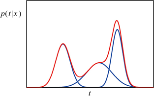
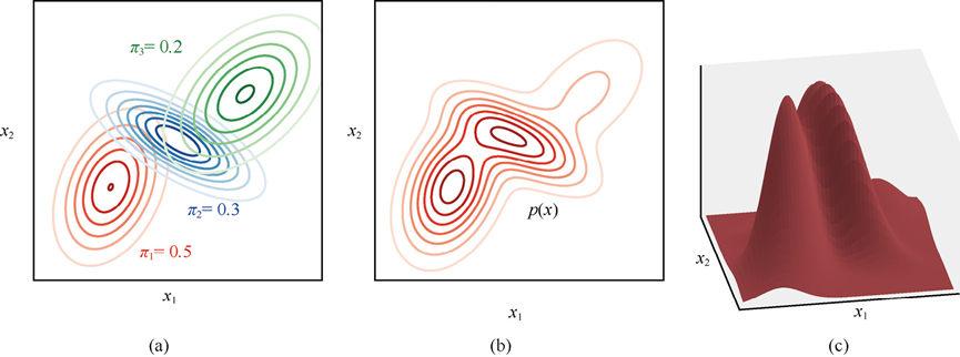
One-dimensional and two-dimensional Gaussian mixtures

Modeling Periodic Variables - von Mises Distribution

Intuition: Imagine a pointer on a clock, wobbling slightly around a certain angle. If you model this with an ordinary Gaussian distribution, the angles $359^\circ$ and $1^\circ$ would be treated as two points far apart, but in reality they are only $2^\circ$ apart. The von Mises distribution is designed for this kind of “circular data”—it is the analogue of the Gaussian distribution defined on a circle.

A periodic variable (such as an angle $\theta \in [0, 2\pi)$) cannot be effectively modeled with a standard Gaussian distribution, because the support (the range of values the variable can take) of the Gaussian distribution is the entire real line, and it cannot handle the periodic connection between $0$ and $2\pi$.

The von Mises distribution is also called the circular normal distribution. Its probability density function is (derivation omitted):

where $\theta_0$ is the mean direction, $m \geq 0$ is the concentration parameter (similar to precision), and $I_0(m) = 1 / 2\pi \int_0^\pi exp(m\cos\theta) d\theta$ is the zeroth-order modified Bessel function, used for normalization. When $m$ is large, the distribution concentrates near $\theta_0$, approximating a Gaussian distribution; when $m=0$, the distribution reduces to the uniform distribution on $[0, 2\pi)$.

Maximum likelihood estimation: For a dataset $\{\theta_1, ..., \theta_N\}$, the maximum likelihood estimate $\theta_{0}^\mathrm{ML}$ of $\theta_0$ satisfies:

This shows that $\theta_{0}^\mathrm{ML}$ is the direction of the centroid of the data points projected onto the unit circle. The maximum likelihood estimate of $m$ requires numerically solving the equation $A(m_{\mathrm{ML}}) = R$, where $R = \sqrt{(\sum \cos \theta_n)^2 + (\sum \sin \theta_n)^2}/N$, and $A(m) = I_1(m)/I_0(m)$.

The von Mises distribution is also unimodal. To model multimodal periodic data, a mixture model of von Mises distributions can be used.

von Mises distribution (left in Cartesian coordinates, right in polar coordinates)

Exponential Family Distributions

Intuition: The Bernoulli, Gaussian, and other distributions discussed earlier look different in shape, but they are actually all “one family”—the exponential family. Just as different drinks (coffee, tea, juice) can all be described using the framework of “water + solute,” the exponential family provides a unified mathematical framework that encompasses most commonly used distributions.

So far, the probability distributions studied are essentially all exponential family distributions (except for mixture models).

The exponential family is a large and important class of probability distributions, whose general form is:

where:

• $\mathbf{\eta}$ is the natural parameter vector (the transformation of the original parameters into the standard form of the exponential family),
• $\mathbf{u}(x)$ is the sufficient statistic vector (contains all the information needed to extract the parameters from the data),
• $h(x)$ is the underlying measure function (usually independent of the parameters),
• $g(\mathbf{\eta})$ is the normalization function, ensuring that the integral of the distribution is 1: $$g(\mathbf{\eta}) = \left[ \int h(x) \exp\left\{ \mathbf{\eta}^\top \mathbf{u}(x) \right\} dx \right]^{-1}$$

It is sometimes also written in the log-normalization form (more common):

where $A(\mathbf{\eta}) = -\ln g(\mathbf{\eta})$ is called the log partition function or cumulant generating function.

In plain terms: The exponential family writes out various common distributions (Bernoulli, Gaussian, Poisson, etc.) using a unified “template.” $\mathbf{\eta}$ is the “natural parameter” after transforming the original parameters (such as the Gaussian’s $\mu, \sigma^2$), $\mathbf{u}(x)$ is the “sufficient statistic” of the data (a function that summarizes all the information in the data), and $A(\mathbf{\eta})$ handles normalization. The benefit of this unified framework is that many properties (such as how to compute the maximum likelihood estimate, and whether a conjugate prior exists) hold for all exponential family distributions, without needing to derive each distribution separately.

Properties:

1. Sufficient statistic (given the dataset, the parameters can be accurately recovered)

• In maximum likelihood estimation, the solution for the parameters depends only on the function of the data $\sum_{n=1}^N \mathbf{u}(x_n)$, without needing to store the entire dataset.
• This means that once $\sum_n \mathbf{u}(x_n)$ is computed, the original data can be discarded, which is very efficient for large-scale data processing.

2. Computation of moments

• The moments (expectation, variance, etc.) of the distribution can be obtained by differentiating $A(\mathbf{\eta})$: $$\mathbb{E}[\mathbf{u}(x)] = \nabla_{\mathbf{\eta}} A(\mathbf{\eta})$$ $$\mathrm{cov}[\mathbf{u}(x)] = \nabla_{\mathbf{\eta}} \nabla_{\mathbf{\eta}}^\top A(\mathbf{\eta})$$
• This makes the computation of expectation and variance systematic and analytically tractable.

3. Existence of conjugate priors

• Every exponential family distribution has a corresponding conjugate prior, such that the posterior distribution belongs to the same family as the prior.

4. Maximum entropy property

• Under given constraints (such as fixing the mean and variance), the exponential family distribution is the distribution with maximum entropy, i.e., the most “uncertain” or most “unbiased” choice.

Examples:

1. Bernoulli distribution

• Let $x \in \{0,1\}$, $p(x|\mu) = \mu^x (1-\mu)^{1-x}$.
• Convert to exponential family form: $$p(x|\eta) = \exp\left\{ \eta x - \ln(1 + e^\eta) \right\}, \quad \text{where } \eta = \ln\left(\frac{\mu}{1-\mu}\right)$$
• Correspondence:
  • $\eta = \ln(\mu/(1-\mu))$ (logit transform),
  • $\mathbf{u}(x) = x$,
  • $h(x) = 1$,
  • $A(\eta) = \ln(1 + e^\eta)$.

2. Univariate Gaussian distribution $\mathcal{N}(x|\mu, \sigma^2)$

• Probability density function: $$p(x|\mu, \sigma^2) = \frac{1}{\sqrt{2\pi\sigma^2}} \exp\left\{ -\frac{(x-\mu)^2}{2\sigma^2} \right\}$$
• Rewrite in exponential family form: $$p(x|\mathbf{\eta}) = \frac{1}{\sqrt{2\pi}} \exp\left\{ \eta_1 x + \eta_2 x^2 - A(\mathbf{\eta}) \right\}$$
• where:
  • Natural parameters: $\mathbf{\eta} = (\eta_1, \eta_2)^\top = \left( \frac{\mu}{\sigma^2}, -\frac{1}{2\sigma^2} \right)^\top$,
  • Sufficient statistic: $\mathbf{u}(x) = (x, x^2)^\top$,
  • Log partition function: $A(\mathbf{\eta}) = -\frac{\eta_1^2}{4\eta_2} + \frac{1}{2}\ln\left(-\frac{1}{2\eta_2}\right)$.

Non-parametric Methods

Intuition: The previous methods all assume that the data follows some specific distribution (such as Gaussian), and then estimate the parameters. Non-parametric methods do the opposite—they do not presuppose the shape of the distribution, but let the data “speak for itself.” It is like using a ruler to measure the outline of an irregular object, rather than first assuming it is circular.

Non-parametric methods do not assume a fixed functional form for the distribution; their complexity (the model’s “degrees of freedom”) typically grows with the amount of data.

Histogram Density Estimation

Divide the range of the variable into fixed-width bins, and the density estimate is the frequency of data points in each bin divided by the bin width and the total amount of data. The advantages are simplicity and intuitiveness; the disadvantages are:

• Sensitive to bin width: too narrow leads to large noise, too wide leads to loss of detail.
• Discontinuity: the density jumps at bin boundaries.
• Curse of dimensionality: in high-dimensional space, most bins are empty.

Histogram density estimation is also a sufficient statistic.

Kernel Density Estimation

Kernel density estimation places a kernel function at each data point (placing a “small hill” around each data point and superimposing all these “small hills” to form the overall density estimate), and then sums them. Its form is:

where $N$ is the number of data points, $D$ is the dimension of the data (for example, for two-dimensional data $D=2$), $h$ is the bandwidth parameter (the width of each “small hill”), controlling the degree of smoothing, and $k(\mathbf{u})$ is the kernel function (which must satisfy non-negativity and an integral of 1). $\frac{1}{h^D}$ ensures that each kernel function integrates to 1 over the entire space (the higher the dimension, the greater the “scaling” required). The Gaussian kernel $k(\mathbf{u}) = \mathcal{N}(\mathbf{u}|\mathbf{0}, \mathbf{I})$ is a common choice.

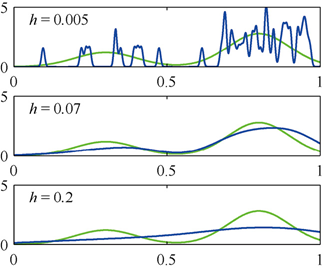
The effect of different bandwidths h on the estimation result in kernel density estimation (too small leads to noise, too large leads to oversmoothing)

The disadvantage is that the cost of evaluating the density at a new point is proportional to the amount of data $N$, which is impractical for large datasets. The choice of bandwidth $h$ is key and affects the degree of smoothing.

K-Nearest-Neighbor Density Estimation

The K-nearest-neighbor method solves the problem of the fixed bandwidth $h$ in kernel density estimation. Its core idea is: near the estimation point $\mathbf{x}$, the sphere centered at $\mathbf{x}$ contains exactly $K$ data points, and the volume $V$ of the sphere is determined by the data. The density estimate is:

where $V$ is the volume of the sphere containing the $K$ nearest neighbors.

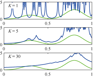
The effect of different K values on the estimation result in K-nearest-neighbor density estimation (the difference between fixed bandwidth and adaptive bandwidth)

The advantage is adaptive smoothing. In dense data regions, $V$ is small, $h$ is small, capturing details; in sparse regions, $V$ is large, $h$ is large, avoiding noise. The disadvantage is again that it needs to store all the data, and computing the density at a new point requires finding the $K$ nearest neighbors, which is costly. When $K$ is small, the estimate may be unstable.

Chapter 3 Summary

One-sentence version: This chapter starts from the simplest “coin flip” (Bernoulli), expands all the way to “rolling a die” (multinomial), the “ellipsoidal cloud” (multivariate Gaussian), “circular data” (von Mises), and finally strings them together with a “unified recipe” (exponential family), followed by the non-parametric methods that “let the data speak for itself.”

Knowledge map:

1
Standard Distributions
2
├── Discrete Variables
3
│   ├── Bernoulli Distribution (coin flip: single binary trial)
4
│   ├── Binomial Distribution (N coin flips: number of successes)
5
│   └── Multinomial Distribution (dice roll: multi-category generalization)
6
├── Continuous Variables
7
│   ├── Univariate Gaussian (one-dimensional bell curve)
8
│   └── Multivariate Gaussian (ellipsoidal cloud)
9
│       ├── Geometry: Mahalanobis distance → equiprobability density surface
10
│       ├── Moments: first = center of gravity, second = spread
11
│       ├── Conditional / Marginal Distributions (cut a slice / project away)
12
│       ├── Bayesian Inference (Gaussian + Gaussian = Gaussian)
13
│       └── Gaussian Mixture Model (multimodal superposition)
14
├── Special Distributions
15
│   ├── von Mises Distribution (circular data)
16
│   └── Exponential Family (unified framework)
17
└── Non-parametric Methods
18
    ├── Histogram (count in grid cells)
19
    ├── Kernel Density Estimation (place a small hill at each point)
20
    └── K-Nearest-Neighbor (adaptive sphere)

Quick-reference table for choosing a distribution:

• Discrete binary data → Bernoulli distribution
• Count data → Binomial or multinomial distribution
• Continuous data assuming normality → Gaussian distribution
• Periodic data → von Mises distribution
• Complex multimodal data → Gaussian mixture model

Chapter 4 Single-Layer Networks: Regression

After the foundations of probability theory in Part 1 and the common probability distributions in Chapter 3 above, this chapter will explore how to use these distributions for actual predictive modeling—which is exactly the foundation of Part 3 (Classification). We will start from the most basic linear regression and gradually build a complete theoretical framework for regression analysis.

Linear Regression

Intuition: Drawing a “best-fit line” on a scatter plot so that the distance from all data points to this line is as small as possible—this is the core idea of linear regression. It predicts one or more continuous target variables $t$ based on a $D$-dimensional input vector (a vector describing sample features) $\mathbf{x}$. Given a training set (training set) containing $N$ observations $\{\mathbf{x}_n\}$ and their corresponding target values $\{t_n\}$, the goal is to predict the value of $t$ for a new input $\mathbf{x}$. This is achieved through a function $y(\mathbf{x}, \mathbf{w})$, where $\mathbf{w}$ is the learnable parameter vector (a model fits the data by adjusting these parameters).

The simplest model is a linear combination of the input variables:

where $\mathbf{x} = (x_1, ..., x_D)^\top$. The key characteristic of this model is its linearity with respect to the parameters $\mathbf{w}$. However, it is also a linear function of the input variables $x_i$, which limits its modeling capacity (it can only learn linear relationships).

Basis Functions

Intuition: If the data is not a straight-line relationship (for example, it is a parabola), fitting directly with a linear model does not work well. The idea of the basis function (basis function) is: first apply a nonlinear transformation to the original input (such as turning $x$ into $x^2$, $e^x$, etc.), and then take a linear combination of the transformed results. It is like straightening a bent wire first, and then measuring it with a ruler.

To expand the model’s capacity (to model nonlinear relationships), we can use a linear combination of fixed nonlinear functions of the input variables:

where $\phi_j(\mathbf{x})$ is called the basis function (a fixed function that applies a nonlinear transformation to the input). The parameter $w_0$ is called the bias parameter, used to handle the fixed offset in the data. Usually, by defining a dummy basis function $\phi_0(\mathbf{x}) = 1$, the model can be written in a more compact vector form:

where $\mathbf{w} = (w_0, ..., w_{M-1})^\top$, $\mathbf{\phi} = (\phi_0, ..., \phi_{M-1})^\top$.

This model can be represented with a simple neural network diagram.

Common basis functions $\phi_j(\mathbf{x})$:

1. Linear basis: $\phi_j(\mathbf{x}) = x_j$
2. Gaussian function: $\phi_j(\mathbf{x}) = e^{-\frac{1}{2s^2} (x_j - \mu_j)^2}$
3. Sigmoid function: $\phi_j(\mathbf{x}) = \frac{1}{1 + e^{- \frac{x -\mu_j} {s}}}$

Maximum Likelihood and Least Squares

Assume the conditional distribution of the target variable $t$ is a Gaussian distribution, with mean equal to the model output $y(\mathbf{x}, \mathbf{w})$ and variance $\sigma^2$:

For an independent and identically distributed (accumulated) dataset, its log-likelihood function (accumulated) is:

Maximizing the log-likelihood is equivalent to minimizing the sum-of-squares error function (see above, Chapter 2 - maximizing the log-likelihood is equivalent to minimizing the sum-of-squares error function):

Substituting the model $y(\mathbf{x}, \mathbf{w}) = \mathbf{w}^\top \mathbf{\phi}(\mathbf{x})$ into the error function $E_D(\mathbf{w})$ above, and taking the derivative with respect to $\mathbf{w}$ and setting it to zero, we obtain the normal equation for the least squares problem:

where $\mathbf{\Phi}$ is the design matrix (each row is a vector of basis function values for one sample), with elements $\Phi_{nj} = \phi_j(\mathbf{x}_n)$.

Pseudo-inverse: When the matrix $\mathbf{\Phi}$ is not full rank / is not square, the least squares solution does not exist. In this case, the least squares solution can be obtained via the pseudo-inverse matrix $\mathbf{\Phi}^\dagger = \mathbf{\Phi}^\top (\mathbf{\Phi} \mathbf{\Phi}^\top)^{-1}$ (in this case, regarded as $\mathbf{\Phi}^\dagger = \mathbf{\Phi}^{-1}$).

Geometric interpretation of least squares:

Intuition: Imagine the target vector $\mathbf{t}$ is a point in space, and the model can only “land” on a certain plane. Least squares finds the point on that plane closest to $\mathbf{t}$—that is, the orthogonal projection (vertical projection) of $\mathbf{t}$ onto the plane.

The least squares solution can be understood as: the model prediction $\mathbf{y} = \mathbf{\Phi} \mathbf{w}$ is the orthogonal projection of the target vector $\mathbf{t}$ onto the linear subspace (the space formed by all linear combinations of the column vectors) spanned by the column vectors of the design matrix $\mathbf{\Phi}$ (i.e., the values of the basis functions at the data points). The error vector $\mathbf{t} - \mathbf{y}$ is orthogonal to this subspace, which is exactly the geometric meaning of the normal equation $\mathbf{\Phi}^\top (\mathbf{t} - \mathbf{\Phi} \mathbf{w}) = \mathbf{0}$.

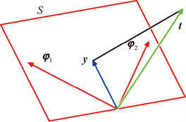
The essence of least squares is to project the true target vector onto the subspace expressible by the model

1. The red plane represents the linear subspace $S$ spanned by the column vectors of the design matrix $\mathbf{\Phi}$. This subspace is the set of all possible model outputs $\mathbf{y} = \mathbf{\Phi} \mathbf{w}$ (i.e., the set of all function values the model can fit). Each column $\phi_j(\mathbf{x}_n)$ is the value of a basis function at a data point, and these vectors together constitute this subspace.
2. The green arrow represents the true target value vector $\mathbf{t}$, pointing from the origin to a point not in the subspace $S$. It represents the true observations we want the model to approximate.
3. The blue arrow $\mathbf{y}$ is the orthogonal projection of $\mathbf{t}$ onto the subspace $S$. It is the result of the model prediction, i.e., $\mathbf{y} = \mathbf{\Phi} \mathbf{w}_{\mathrm{ML}}$. The goal of least squares is to find such a $\mathbf{y}$ so that it is as close as possible to $\mathbf{t}$.
4. The black arrow represents the residual (error) $\mathbf{e}$, i.e., the gap between the actual value and the predicted value. It is perpendicular to the subspace $S$, indicating that the error vector is orthogonal to any direction in the subspace. This is exactly the core meaning of the normal equation: $\mathbf{\Phi}^\top (\mathbf{t} - \mathbf{\Phi} \mathbf{w}) = \mathbf{0}$ (i.e., the error vector is orthogonal to the directions of all basis functions).
5. $\varphi_1$ $\varphi_2$ represent the basis functions, with elements $\phi_j(\mathbf{x}_n)$.

Sequential Learning

Intuition: The normal equation above needs to “swallow” all the data at once to compute the result. If the amount of data is huge or the data keeps arriving continuously, what do we do? The strategy of Stochastic Gradient Descent (SGD) is: for each data point that arrives, slightly adjust the parameters in the direction of decreasing error, just like adjusting your direction with each step as you go down a mountain.

When the dataset is large or data arrives in a streaming fashion, batch-processing all the data to compute $\mathbf{w}_{\mathrm{ML}}$ may be impractical. Here we can use Stochastic Gradient Descent (SGD) for sequential learning. For the sum-of-squares error function, the SGD update rule is:

($\nabla E$ uses the sum-of-squares error function above) where $\mathbf{\phi}_n = \mathbf{\phi}(\mathbf{x}_n)$, and $\eta$ is the learning rate. This is called the Least Mean Squares (LMS) algorithm.

Regularized Least Squares

In Part 1 we discussed: to prevent overfitting (the model adapts too closely to the noise in the training data, leading to poor performance on new data), especially when there are many basis functions or little data, a regularization term (an additional term that penalizes model complexity) can be added to the error function. The simplest form is L2 regularization (L2 regularization, also called weight decay, which penalizes the sum of squares of the parameters):

The solution obtained by minimizing this function is:

The regularization term ensures that the matrix $(\mathbf{\Phi}^\top \mathbf{\Phi} + \lambda \mathbf{I})$ is always invertible, even when $\mathbf{\Phi}^\top \mathbf{\Phi}$ is singular. (It is an extension of $\mathbf{w}_{ML}$; see above, $\mathbf{w}_{ML}$ - normal equation for least squares problem)

Decision Theory

Intuition: You predict that tomorrow’s temperature is $25^\circ C$, but it is actually $23^\circ C$. How much did this prediction “miss” by? What does a difference of $2^\circ C$ mean in terms of cost? Decision theory is the framework that answers “how to make optimal predictions based on a probabilistic model”; see Part 3 (Classification) for further discussion.

The next chapter will also explain in detail

Decision theory guides us on how to make optimal predictions based on a probabilistic model. For regression problems, we use a loss function (a function that quantifies the “cost” between the prediction and the true value) $L(t, y(\mathbf{x}))$ to quantify the cost between the prediction $y(\mathbf{x})$ and the true value $t$. The goal is to choose the prediction function $y(\mathbf{x})$ to minimize the expected loss:

For the squared loss $L(t, y) = \{y - t\}^2$, the optimal prediction function that minimizes the expected loss is the conditional mean:

Be careful not to confuse the error function with the loss function. The error function is used to set the parameters during training, while the loss function is used to control how to use the conditional distribution to arrive at the prediction function f(x) for predicting x, which is exactly what the linear regression model tries to learn.

The expected loss can be decomposed into two parts:

The first term is the mean squared error between the prediction function and the true regression function (which can be reduced by improving the model), and the second term is the variance of the target variable given the input (irreducible error, the noise that cannot be eliminated no matter how good the model is).

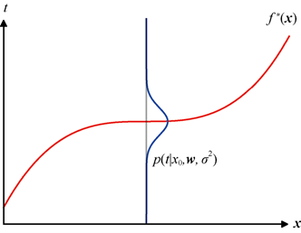
The regression function that minimizes the squared loss is given by the mean of the conditional distribution

Other loss functions:

• Minkowski loss: $L_q = |y - t|^q$.
• $q=2$: the optimal solution is the conditional mean.
• $q=1$: the optimal solution is the conditional median.
• $q \to 0$: the optimal solution is the conditional mode.

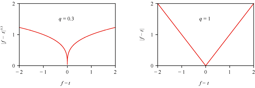
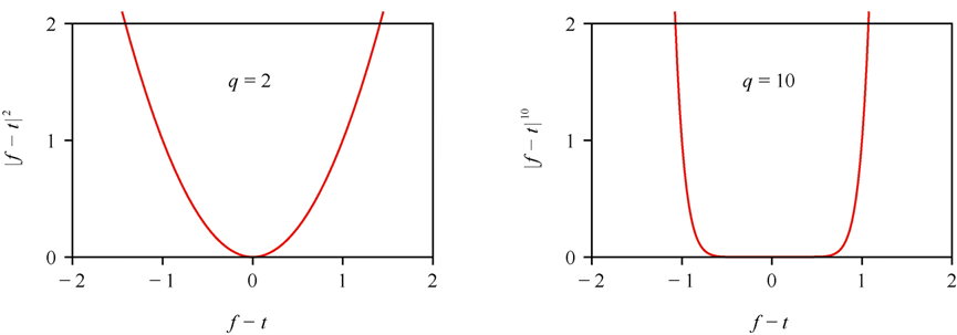
Effect of different values of q

Bias-Variance Tradeoff

Intuition (target shooting metaphor): Imagine you are shooting at a target.

• Bias is whether your gun sight is aimed accurately—if the scope is crooked, all the bullets will deviate from the bullseye, but the holes will be tightly clustered.
• Variance is whether your hand is shaking—even if the scope is fine, a shaky hand will scatter the bullet holes around the bullseye.
• High bias + low variance = crooked scope but steady hand (simple model, underfitting)
• Low bias + high variance = straight scope but shaky hand (complex model, overfitting)
• Best = straight scope and steady hand (the balance point between bias and variance)

In model selection, there is a tradeoff between bias (the systematic prediction error of the model) and variance (the sensitivity of the model to changes in the training data). Bias measures the systematic deviation of the model’s average prediction from the true function. Variance measures the sensitivity of the model’s predictions to a specific training dataset.

Consider a simple regression problem, where the true function is $f(x)$, and the observed data is generated by $t = f(x) + \epsilon$, with $\epsilon$ being zero-mean noise. A model $y(x; \mathcal{D})$ (dependent on the dataset $\mathcal{D}$) is used for prediction. The expected prediction error can be decomposed as:

where $\bar{y}(x) = \mathbb{E}_\mathcal{D}[y(x; \mathcal{D})]$ is the average prediction of the model over different datasets (imagine training the same model with infinitely many different training sets and taking the average of the predictions).

• High bias, low variance (crooked scope but steady hand when shooting): a simple model (such as a low-degree polynomial) may fail to capture the complexity of the data, leading to high bias, but its predictions are insensitive to changes in the dataset (low variance) -> underfitting (the model is too simple and hasn’t even learned the patterns in the training data)
• Low bias, high variance (straight scope but shaky hand when shooting): a complex model (such as a high-degree polynomial) can fit the training data well (low bias), but may overfit the noise in the training data, leading to large prediction differences across different datasets (high variance) -> overfitting

The optimal model strikes a balance between bias and variance to minimize the total error. This tradeoff is the theoretical foundation of the model selection problem in Part 1, and will appear again in Part 3 (Classification).

Bias-variance tradeoff (variance grows larger on the left, bias grows smaller on the right)

Chapter 4 Summary

One-sentence version: Linear regression = drawing the best-fit line on a scatter plot; decision theory = tells you how “best” is defined (minimize loss); bias-variance tradeoff = a model that is too simple underfits, too complex overfits, and you need to find a balance.

Knowledge map:

1
Single-Layer Networks: Regression
2
├── Linear Regression
3
│   ├── Basic model: y = w^T x (draw a straight line)
4
│   ├── Basis function extension: y = w^T phi(x) (draw a curve)
5
│   ├── Parameter learning
6
│   │   ├── Maximum likelihood ≡ Least squares (normal equation)
7
│   │   ├── Geometric interpretation: orthogonal projection
8
│   │   └── Sequential learning: SGD / LMS
9
│   └── Regularization: L2 weight decay (prevent overfitting)
10
├── Decision Theory
11
│   ├── Loss function: quantifies prediction cost
12
│   ├── Squared loss → optimal prediction = conditional mean
13
│   └── Expected loss = reducible error + irreducible error
14
└── Bias-Variance Tradeoff
15
    ├── Bias: is the scope accurate (systematic error)
16
    ├── Variance: is the hand shaking (sensitivity to data)
17
    └── Optimal model = balance point between bias and variance