Part 1/8 of the series → Next | Glossary

This series has 8 parts in total. It is recommended to read them in order, but if you are short on time:

• To understand the basic concepts: read Parts 1-3
• To understand how neural networks are trained: read Part 4
• To learn about mainstream architectures: read Part 5-Part 6
• To understand generative models: read Part 7-Part 8
• Encounter an unfamiliar term? Check the Glossary

Prerequisites: In theory, high school math is sufficient, and a foundation in calculus is preferable. If you know what a function is and what a derivative is, you can follow along. Goal of this part: After reading, you will understand—what overfitting is, how regularization works, and the most core concepts of probability theory and information theory.

Reference book: “Deep Learning: Foundations and Concepts” (2025) - by Christopher M. Bishop and Hugh Bishop

Chapter 1 Deep Learning Preliminaries: From Drawing a Line to Neural Networks

Fitting a Line Through a Bunch of Points

Imagine you have a scatter plot (say, the relationship between house area and price), and you want to draw a line to describe the pattern. How do you measure whether the line is drawn well?

The error function does exactly this: square the difference (error) between the actual value $t_n$ of each data point $x_n$ and the predicted value $y(x_n,w)$ of your drawn line, sum them all up, and then divide by 2—this gives you a score of “how good the line is drawn”, where a smaller score means a better fit.

In plain words: error function = half the sum of the squares of each point’s “deviation”.

where $(y(x_n,w) - t_n)^2$ is the prediction error of the $n$-th point.

The polynomial function (the line you drew) is:

The error function is always ≥ 0 (because it is a sum of squares). Our goal is to find the set of parameters $w$ that minimizes this function, denoted as $w^*$. How do we find it? Take the derivative of $E(w)$, set it to 0, and the resulting $w$ is $w^*$.

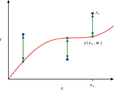
Green is the error, red is the prediction function, blue is the true value

Model Complexity: Neither Too Simple Nor Too Complex Works

Choosing the order of the polynomial (model complexity) is a profound matter:

• Underfitting: The model is too simple and fails to learn even the basic pattern of the data (e.g., using a straight line to fit data that is parabolic in shape).
• Overfitting: The model is too complex and also learns the noise (random fluctuations) in the data as if it were a pattern, causing poor performance on new data (e.g., using a 10th-order polynomial to fit data that is inherently 2nd-order, causing the curve to oscillate violently).

How do we judge whether it is overfitting? Split the data into a training set (used to fit the model) and a test set (used to evaluate the model), and use the root mean square error to assess it:

This formula does two things: dividing by $N$ allows datasets of different sizes to be compared fairly, and taking the square root makes the error unit consistent with the original data (e.g., house prices in “yuan” rather than “yuan²”).

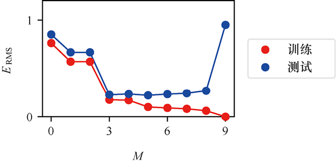
The higher the order, the more complex the model, and the more prone it is to overfitting; the lower the order, the more prone it is to underfitting

This is intuitive: the higher the order, the more “flexible” the curve, and the more easily it is led astray by random noise in the data, and the coefficients also become very large. At the same time, the larger the amount of data, the more it can support a complex model—this is like an exam with more questions, where it is harder to get things right by luck.

In short: model complexity must match the amount of data. With little data, use a simple model; only with a lot of data can you use a complex model.

Regularization: Putting a “Tightening Spell” on the Model

You might ask: since overfitting is caused by the parameters $w$ being too large, making the model too complex, can we just directly restrict the size of $w$?

Exactly! This is the idea of regularization. The approach is simple: add a penalty term after the original error function, penalizing whoever has a large $w$:

This penalty term is also called weight decay, because it keeps “shrinking” the parameters $w$. From a probability theory perspective (detailed in Chapter 2 later), this is equivalent to placing a Gaussian prior with mean 0 on the parameters $w$—meaning we assume in advance that the parameters should be relatively small.

The key lies in the size of $\lambda$ (lambda, the regularization coefficient):

• $\lambda$ larger → heavier penalty → smaller $w$ → simpler model → more prone to underfitting
• $\lambda$ smaller → lighter penalty → larger $w$ → more complex model → more prone to overfitting

How do you choose $\lambda$? Try different values of $\lambda$ on a validation set and see which one gives the smallest $E_{RMS}$.

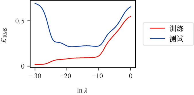
Root mean square error on the validation set vs λ

In short: regularization is like putting a tightening spell on the model—want the parameters to grow? First ask whether $\lambda$ agrees.

Cross-Validation: How to Evaluate a Model Fairly?

Above we said to use a validation set to select $\lambda$, but the question is: how do we partition the validation set? If it is too large, there is not enough training data; if too small, the evaluation is inaccurate.

S-fold cross-validation is a clever solution:

1. Randomly split the data into $K$ parts (e.g., K=4)
2. Round 1: train on parts 2, 3, 4 and validate on part 1; Round 2: train on parts 1, 3, 4 and validate on part 2… and so on
3. After running $K$ rounds, average all the validation errors

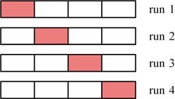
S-fold with K=4, red is the validation set

This way, every part of the data serves as the validation set once, making the evaluation result more reliable. The cost is that training is done $K$ times more.

Special case: when $K=N$ (the size of the dataset), only 1 sample is left out for validation each time, which is called leave-one-out.

S-fold cross-validation is often used to select the hyperparameters of neural networks (hyperparameter, i.e., parameters that need to be set manually before training, such as the number of hidden layer nodes and the learning rate), avoiding dependence on any particular partition.

Neural Networks: Starting from a “Switch”

When the data relationship is very complex (highly nonlinear), polynomial fitting requires a high order and is prone to overfitting. Is there a better method?

The neural network is the answer. Its inspiration comes from the human brain: neurons connect through synapses, receiving, processing, and outputting signals. We start from the simplest “neuron”:

A neuron does three things:

1. Receive input: multiply each input $x_1, x_2, \cdots, x_n$ by a weight $w_1, w_2, \cdots, w_n$ respectively, and add them up—this gives the pre-activation (the weighted sum before passing through the activation function).
2. Activate: transform the pre-activation value through an activation function nonlinearly.
3. Output: obtain the result of this neuron.

Common activation functions include sigmoid (an S-shaped curve that compresses any value into the range 01), tanh (similar to sigmoid but with output range -11), and ReLU (negative values become 0, positive values unchanged, the preferred choice for modern deep networks).

Analogy: dendrites receive input signals → cell body processes (activation) → axon outputs the result.

The simplest neural network is the perceptron—it has only a single neuron, and its activation function is a “switch”:

The modern multi-layer perceptron (MLP) stacks many such “switches” into multiple layers, where the output of each layer serves as the input of the next, passing information layer by layer until the final result is obtained. The more layers there are, the more complex the patterns that can be learned—this is the origin of the word “deep” in “deep learning”.

Chapter 1 Summary

One-sentence version:

• Error function: measures how far the model’s line is from the data points; the smaller the better.
• Overfitting: the model is too complex and treats noise as a pattern; Underfitting: the model is too simple and fails to learn the pattern.
• Regularization: adds a penalty term to the parameters to prevent the model from being too complex.
• Cross-validation: splits the data into multiple parts for training and validation in rotation, to evaluate the model fairly.
• Neural network: a bunch of simple “switches” stacked into multiple layers, capable of learning very complex patterns.

Knowledge map:

1
Error function → Overfitting/Underfitting → Regularization + Cross-validation
2
                              ↓
3
        Limitations of polynomial fitting → Neural Networks (MLP)

In the next chapter we will learn probability theory—it is the mathematical foundation for understanding “why the error function looks like this” and “how the model makes predictions”.

Chapter 2 Probability: Reasoning Under Uncertainty

Why do we need probability? Because the real world is full of uncertainty.

There are two kinds of uncertainty:

• Aleatoric uncertainty: the data itself has noise, such as measurement instrument errors and natural fluctuations in human height—this cannot be eliminated.
• Epistemic uncertainty: because we have not collected enough data, our understanding of the pattern is incomplete—the more data, the smaller this kind of uncertainty.

Probability theory is the mathematical language for dealing with uncertainty. Many core concepts of deep learning (maximum likelihood estimation, cross-entropy, KL divergence) are built on top of probability theory.

Prerequisites: knowing what “probability” is is sufficient.

Two Schools of Thought: What Exactly Is Probability?

Starting from a coin: the probability of heads is 0.5—but what does this sentence really mean?

The frequentist view holds that probability is “the frequency with which something occurs after repeating the experiment many times”. You toss a coin 1000 times, roughly 500 heads, so the probability is 0.5. Parameters (such as the coin’s weight distribution) are fixed but unknown, and we use data to estimate them.

• Representative methods: maximum likelihood estimation (MLE), confidence intervals.

The Bayesian view holds that probability is “our degree of belief that something will happen”. Before you toss the coin, but based on experience you think it is roughly half and half—this is the prior belief; after tossing a few times, you update this belief based on the results.

• Key formula: Bayes’ theorem (explained below).

Both views have their merits and are both applied in deep learning. Frequentist methods are more common (such as maximum likelihood estimation), but Bayesian thinking is also important in regularization and uncertainty estimation.

Probability Basics: Three Iron Laws

There are only three probability rules; just remember them:

Sum rule: to know the probability that $X = x_i$, sum the probabilities of $X = x_i$ over all possible values of $Y$:

Product rule: the probability that two events occur together = the probability that the first occurs × the probability that the second occurs given that the first has occurred:

Bayes’ theorem: this is the most important one—it tells us how to reason backward from “effect” to “cause”:

In plain words: posterior probability = (likelihood × prior) / evidence

• Prior probability $P(Y)$: our belief about $Y$ before observing $X$.
• Posterior probability $P(Y|X)$: the updated belief about $Y$ after observing $X$.
• Likelihood $P(X|Y)$: the probability of observing $X$ if $Y$ is true.
• Evidence $P(X)$: a normalization constant ensuring the probabilities sum to 1.

Example: you see the ground is wet ($X$) and want to judge whether it rained ($Y$). Prior $P(Y)$: according to the weather forecast, the probability of rain is 30%. Likelihood $P(X|Y)$: if it rained, the probability the ground is wet is 90%. Likelihood $P(X|\neg Y)$: if it did not rain, the probability the ground is wet is 10% (maybe a sprinkler truck). Posterior $P(Y|X)$: after seeing the ground is wet, what is the actual probability it rained? Use Bayes’ theorem to compute it.

Independence: if two variables $X$ and $Y$ do not affect each other, $P(X, Y) = P(X)P(Y)$.

Probability Density: Probability for Continuous Variables

For discrete variables (such as dice points), each value has a definite probability. But for continuous variables (such as height, temperature), the probability of taking any exact value is 0—can you be exactly 170.000000… cm tall? Impossible.

So we introduce the probability density function (PDF) $p(x)$: it means the probability that $x$ falls in a small interval $(x, x+\delta x)$ is approximately $p(x)\delta x$.

The probability that $x$ falls in the interval $(a, b)$ is the area under the density curve in that interval:

The probability density function must satisfy two conditions:

• Non-negativity: $p(x) \geq 0$ (probability cannot be negative).
• Normalization: $\int_{-\infty}^{\infty} p(x) dx = 1$ (the total probability must be 1).

The cumulative distribution function (CDF) $P(z) = \int_{-\infty}^z p(x) dx$ means “the probability that $x$ is less than or equal to $z$”. Its derivative is the probability density: $P'(x) = p(x)$.

The sum rule and product rule above apply equally to continuous variables, just replacing summation with integration:

• Sum rule: $p(\mathbf{x}) = \int p(\mathbf{x}, \mathbf{y}) d\mathbf{y}$ (integrate out the variables we do not care about).
• Product rule: $p(\mathbf{x}, \mathbf{y}) = p(\mathbf{y}|\mathbf{x})p(\mathbf{x})$.

Bayes’ theorem is likewise:

The above rules apply equally ($\mathbf{x}, \mathbf{y}$ are two real-valued variables, multivariate/multi-dimensional):

Sum rule - when interested in only part of the variables, integrate out the other variables to obtain the distribution of the variables of interest

Product rule - when considering dependencies between variables, the joint distribution can be decomposed into the product of the conditional and marginal distributions

Bayes’ theorem

The denominator (marginal probability) can likewise be written as:

Common Probability Distributions

Before diving into deep learning, let us get to know several of the most commonly used probability distributions. You can think of them as “LEGO bricks”—many complex probabilistic models are assembled from these basic distributions.

Uniform distribution: the simplest kind—within the finite interval $(c, d)$ the probability density is equal everywhere, like pouring water evenly into a flat-bottomed container:

Exponential distribution: the probability density monotonically decreases starting from some point, often used to model “waiting time” (e.g., how long to wait for a bus):

where the larger $\lambda$ (lambda) is, the faster the decay, indicating a higher probability of “being able to wait soon”.

Laplace distribution: looks like two exponential distributions back to back, centered at $\mu$ with a sharp peak. It is “sharper” than the Gaussian distribution and has “heavier” tails, making it more robust to outliers:

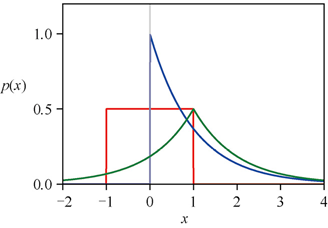
Red is the uniform distribution, blue is the exponential distribution, green is the Laplace distribution

The next two distributions are special; they are not ordinary “curves” but very useful tools in probability theory and statistics:

Dirac delta function: this is not an ordinary function but a kind of “generalized function”—you can imagine it as an infinitely thin, infinitely tall “needle” stuck at $x = \mu$, but the area under this needle is exactly 1:

It is zero everywhere except at $x = \mu$, but $\int p(x|\mu) dx = 1$. It frequently appears in physics and probability theory to represent “precisely determined at some position”.

Empirical distribution: given a set of real data $D = \{x_1, \ldots, x_N\}$, the empirical distribution uses this very data itself to “approximate” the true distribution—the approach is simple: stick a δ-function “needle” at each data point $x_n$, each needle having height $\frac{1}{N}$:

In plain words: you have 10 observed data points, and the empirical distribution says “each data point has probability 1/10, and 0 everywhere else”. It is the most naive way of “letting the data speak for itself”.

Expectation and Variance

Expectation

In plain words, expectation is the theoretical version of the “weighted average”. Normally you compute the average by summing all the data and dividing by the count; expectation instead multiplies each value by the probability of its occurrence and then sums—taking into account “how likely each value is to occur”.

Discrete case: multiply each value by its corresponding probability and sum

Continuous case: replace summation with integration

Finite samples: when you only have a finite number of data points, use the empirical distribution to approximate—this is the “stick a needle at each data point” approach mentioned earlier. Specifically, using the property of the δ-function ($\int \delta(x - x_n) f(x) dx = f(x_n)$) it simplifies to:

In short: the sample mean is an approximation of the expectation. The more data, the more accurate the approximation. This is exactly the core idea of Chapter 14 - Monte Carlo approximation.

Conditional expectation: the expectation of $f(x)$ after knowing the value of some variable $y$—the result is a function of $y$:

Variance

Variance measures “how spread out the data is around the expectation”—in simple terms, “how large the fluctuation is”. The larger the variance, the more dispersed the data; the smaller the variance, the more concentrated the data is around the mean.

where $E[f(x)^2]$ is the “expectation of the square” and $E[f(x)]^2$ is the “square of the expectation”—variance is the difference between the two.

The variance of the variable $x$ itself is the special case for $f(x) = x$:

Covariance

Covariance measures the “tendency of two variables to change together”. If $y$ tends to increase when $x$ increases, the covariance is positive; if one increases while the other decreases, the covariance is negative; if they do not affect each other it is 0.

If $x$ and $y$ are independent, then $\text{cov}[x, y] = 0$ (note that the converse does not hold—zero covariance does not imply independence, there could be a nonlinear relationship).

Vector covariance: for vectors $\mathbf{x}$ and $\mathbf{y}$, the covariance is a matrix:

The covariance matrix of the vector $\mathbf{x}$ itself describes the correlations between its components—the diagonal holds the variances and the off-diagonal holds the covariances.

Gaussian Distribution (Normal Distribution)

The Gaussian distribution, also called the normal distribution, is the most important distribution in probability theory, bar none. Its shape is a symmetric bell curve—high in the middle, low on both sides, symmetric left and right.

Gaussian distribution → maximum likelihood estimation → derivation of the loss function for linear regression → the meaning of noise modeling

This thread runs through the next few subsections; as you read, keep this question in mind: why is the Gaussian distribution so important?

Univariate Gaussian Distribution

The formula looks intimidating, but in fact only two parameters control everything:

• $\mu$ (mu, mean): determines the center position of the bell curve—where the highest point of the curve is.
• $\sigma^2$ (sigma squared, variance): determines the width of the bell curve—the larger $\sigma$ is, the “fatter” and “shorter” the curve; the smaller $\sigma$ is, the “skinnier” and “taller” the curve.
• $\sigma$ (standard deviation): the square root of the variance, describing the same thing as the variance, but with a unit consistent with the original data.
• $\beta = 1/\sigma^2$ (precision): the reciprocal of the variance; the larger the precision, the more concentrated the distribution.

Of course, as a probability density function, it must satisfy:

Properties of the Gaussian Distribution

• Expectation (first moment): $E[x] = \mu$—the “center of mass” of the distribution is at the mean. For the concept of moments, see Chapter 3 - Moments.
• Second moment: $E[x^2] = \mu^2 + \sigma^2$.
• Variance: $\text{var}[x] = E[x^2] - E[x]^2 = \sigma^2$.
• Mode (the position of the maximum probability density): for the Gaussian distribution, the mode coincides with the mean $\mu$—the highest point is right in the middle.

A Probabilistic View of Linear Regression

Remember the linear regression and error function from Chapter 1? Now we can re-understand it in the language of probability.

Model the regression problem as a conditional probability: the target value $t$ is a random variable that follows a Gaussian distribution centered at the predicted value $y(x, \mathbf{w})$:

where $y(x, \mathbf{w})$ is the model’s prediction and $\sigma^2$ is the noise variance.

Imagine you are predicting house prices: the input $x$ is the house area, and the model predicts $y(x, \mathbf{w})$ as the predicted price. The actual price $t$ will not equal the predicted price exactly—it fluctuates randomly around the predicted price (because factors like school district and decoration are not accounted for).

The probabilistic view says: this fluctuation follows a Gaussian distribution. That is, the house price $t$ follows a Gaussian distribution with mean equal to the predicted value $y(x, \mathbf{w})$. What is the benefit? When predicting, you can output an interval (e.g., $y \pm 2\sigma$) instead of a single isolated number—this quantifies the uncertainty.

Likelihood Function

What Is Likelihood?

Imagine you are playing a “guess the parameter” game: I give you a dataset (say, the heights of 10 people), tell you the data comes from a Gaussian distribution, but do not tell you the mean and variance. Your task is: guess a set of parameters that maximizes the probability that “this dataset occurs”.

This “probability that the data occurs” is the likelihood function. Given the parameters $\mu$ and $\sigma^2$, the likelihood of observing the dataset $\mathbf{x} = (x_1, \ldots, x_N)$ is:

You might ask: why multiply? Because we assume the data is independent and identically distributed (i.i.d.)—each data point is independently drawn from the same distribution, so the joint probability is the product of the individual probabilities.

Log-Likelihood

Multiplying is troublesome (numerically prone to overflow), so we usually take the logarithm, turning the product into a sum:

Maximum Likelihood Estimation (Maximum Likelihood, ML)

Maximum likelihood estimation (MLE) is the answer to the “guess the parameter” game—find the set of parameters that maximizes the likelihood function. The approach is: take the derivative of the likelihood function (or log-likelihood), set it to 0, and solve for the parameters.

For the Gaussian distribution, the result is surprisingly simple:

• Maximum likelihood solution for the mean $\mu$: it is the sample mean $$\mu_{ML} = \frac{1}{N} \sum_{n=1}^N x_n$$
• Maximum likelihood solution for the variance $\sigma^2$: it is the sample variance $$\sigma^2_{ML} = \frac{1}{N} \sum_{n=1}^N (x_n - \mu_{ML})^2$$

In plain words: want to know a group of people’s average height and the range of height variation? Taking the average of their heights gives $\mu_{ML}$, and computing the average of the squared deviations of each person from the mean gives $\sigma^2_{ML}$.

Bias of Maximum Likelihood Estimation

Here is a subtle but important issue: the maximum likelihood estimate of the variance is biased.

For the Gaussian distribution:

• $E[\mu_{ML}] = \mu$ (the mean estimate is unbiased—exactly right)
• $E[\sigma^2_{ML}] = \frac{N-1}{N} \sigma^2$ (the variance estimate is biased—it systematically underestimates the true variance)

Why is the variance underestimated? Imagine you are predicting height:

1. If you knew the true average height, you could directly compute the variance using this value.
2. But you do not—you can only use the sample mean $\mu_{ML}$ computed from the same dataset as a substitute.
3. The sample mean is computed from the same dataset, so it is naturally “closer” to this dataset than the true mean.
4. Therefore the computed variance is a bit too small—this is like “grading yourself”, which always scores a bit higher than others would.

Correction method: use $N-1$ instead of $N$ in the denominator to obtain the unbiased variance estimator:

In short: as the amount of data $N$ increases, $\frac{N-1}{N}$ gets closer and closer to 1, and the bias gets smaller and smaller. But in complex models (such as neural networks), the data is often insufficient relative to the number of parameters, and the bias problem of maximum likelihood (closely related to overfitting) becomes more severe.

Maximum Likelihood Estimation = Minimizing the Sum-of-Squares Error

Remember the error function from Chapter 1? Now we can understand it from a probabilistic perspective.

When we model the regression problem with a Gaussian distribution, maximizing the likelihood function:

After taking the logarithm we obtain the log-likelihood function. The term $-\frac{N}{2}\ln(2\pi\sigma^2)$ does not depend on $\mathbf{w}$, so we only need to maximize:

Because $\sigma^2 > 0$ is a constant, this is equivalent to minimizing the sum-of-squares error function:

This is why the sum-of-squares error is the default loss function for regression problems—it is not designed out of thin air, but is the natural result of maximum likelihood estimation when assuming the noise follows a Gaussian distribution.

In other words: the least squares method = maximum likelihood estimation under the Gaussian noise assumption.

Prediction Distribution

With the maximum likelihood estimates of the parameters, we can write out the complete prediction distribution. The maximum likelihood estimate of the noise variance is:

The prediction distribution is:

Example of predicting height:

• Input: age $x = 10$ years
• Model prediction: $y(10, \mathbf{w}) = 140$ cm
• Maximum likelihood estimate of the noise variance: $\sigma^2 = 25$ (standard deviation $\sigma = 5$ cm)
• Distribution of the actual height $t$: $p(t|x=10) = \mathcal{N}(t|140, 25)$
• So we can expect the actual height to be roughly in the range 130~150 cm (mean $\pm 2$ standard deviations, covering about 95% of the probability)

Variable Transformation

You might ask: how does the probability density change under a variable transformation? It is not simply a matter of “replace $x$ with $y”—the transformation of probability density is different from that of ordinary functions.

Starting with Intuition: Stretching a Rubber Band

Imagine you uniformly apply ink (uniform probability density) on a rubber band. Now you stretch the rubber band to twice its original length—the ink is “diluted” and the density becomes half of the original. But the total amount of ink (probability) has not changed.

Simple example: linear transformation $x = 2y$ In $y$-space, the length of the interval $[0, 1]$ is 1; in $x$-space it becomes $[0, 2]$, with length 2. If $p_y(y) = 1$ (in the interval $[0,1]$), then $p_x(x)$ in the corresponding interval should be $1/2$—so that the total probability is conserved: $\int_0^1 p_y(y) dy = \int_0^2 p_x(x) dx = 1$

Nonlinear Variable Transformation

For linear transformations, the scaling factor is constant. But for nonlinear transformations, the “stretching ratio” differs at every position—just like the stretching is different at different positions of the rubber band.

Consider a small interval $[y, y+dy]$, whose probability in $y$-space is $p_y(y) dy$ (remember the probability density function?).

After the transformation $x = g(y)$, this interval becomes $[x, x+dx]$, where $dx = g'(y) dy$. To preserve probability conservation (the probability before and after the transformation must be equal):

Therefore:

The absolute value is taken because the probability density must be non-negative. Here $\left|\frac{dg}{dy}\right|$ is the Jacobian factor—in one dimension it is just the absolute value of the derivative, representing the scaling ratio of the interval length before and after the transformation.

Univariate Transformation Formula

Let $x = g(y)$, then the probability density of the new variable $y$ is:

The Mode Position Changes!

The mode is the point where the probability density function reaches its maximum (for the Gaussian distribution it is the mean). There is an easy mistake to make here:

If we simply assume $p_y(y) = p_x(g(y))$ (ignoring the Jacobian factor), we would think the mode is just a coordinate transformation—the mode of $p_x$ is at $\hat{x}$, and after transformation the mode of $p_y$ is at $\hat{y}$ satisfying $\hat{x} = g(\hat{y})$.

But this is wrong! Because there is an extra $\left|\frac{dg}{dy}\right|$ term in the formula, its derivative introduces an additional term, causing the mode position to shift.

For example: suppose $p_x(x) = \mathcal{N}(x|1, 0.5^2)$ (mode at $x = 1$), and apply the nonlinear transformation $x = g(y) = y^3$:

• Naive expectation: ignoring the Jacobian, think the mode is at $y = 1$ (because $1^3 = 1$).
• Correct transformation: $p_y(y) = p_x(y^3) \cdot \left|\frac{d(y^3)}{dy}\right| = p_x(y^3) \cdot |3y^2|$ Due to the extra $3y^2$ term, the position of the maximum of $p_y(y)$ shifts and no longer satisfies $\hat{x} = g(\hat{y})$.

This conclusion can be verified by sampling: after sampling $x$ and transforming to $y$, the histogram of $y$ matches $p_y(y)$, not $p_x(g(y))$.

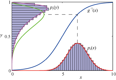
The result should be the red curve, not the green curve; the maxima (modes) do not match

Note: under a linear transformation, the Jacobian factor is a constant, and this problem disappears—the transformation of the mode position is as expected.

Transformation of Multivariate Distributions

Let $\mathbf{x} = \mathbf{g}(\mathbf{y})$ ($\mathbf{x}$, $\mathbf{y}$ are both $D$-dimensional vectors), the transformation formula is:

where $\mathbf{J}$ is the Jacobian matrix, with elements $J_{ij} = \frac{\partial g_i}{\partial y_j}$.

$|\det \mathbf{J}|$ is the absolute value of the determinant of the Jacobian matrix—you can think of it as the multi-dimensional version of “rubber band stretching”: originally there is a small square in $(y_1, y_2)$-space, which after transformation becomes an irregular quadrilateral in $(x_1, x_2)$-space, and $|\det \mathbf{J}|$ is the scaling factor of the area (or volume).

Variable transformation is very important in deep learning—the core idea of normalizing flow models is to progressively transform a simple distribution (such as a Gaussian distribution) into a complex distribution through a series of invertible transformations. Each transformation needs to be multiplied by the Jacobian factor.

Entropy

Information Content: A “Surprise Meter”

Imagine you are a news editor. Of the following two pieces of news, which is more “newsworthy”?

• “Tomorrow the sun rises in the east”—probability almost 100%, no surprise at all.
• “Tomorrow the sun rises in the west”—probability almost 0%, super shocking.

Intuition tells us: the less likely an event is, the more information its occurrence carries. This is the core idea of information content.

The information content function $h(x)$ should satisfy two conditions:

1. The lower the probability, the greater the information content; for an event with probability 1, the information content is 0.
2. The information content of two independent events occurring together = the sum of their individual information contents (additivity).

The function satisfying these two conditions is the logarithm of the probability (the negative sign ensures non-negativity):

When the base is 2, the unit is bits.

Entropy: Average Information Content

Entropy $H[x]$ is the expectation (average) of the information content—it measures how “uncertain” or “chaotic” a random variable is overall:

When $p(x) = 0$, define $p(x) \ln p(x) = 0$ (because $\lim_{x \to 0} x \ln x = 0$).

Examples:

1. Uniform distribution: 8 equally probable states, each with probability $1/8$. Entropy $H[x] = -8 \times \frac{1}{8} \log_2 \frac{1}{8} = 3$ bits.

   Because each state is equally likely, you cannot guess at all what the next one will be—maximum uncertainty.

2. Non-uniform distribution: states $\{a, b, c, d, e, f, g, h\}$ have probabilities $\{\frac{1}{2}, \frac{1}{4}, \frac{1}{8}, \frac{1}{16}, \frac{1}{64}, \frac{1}{64}, \frac{1}{64}, \frac{1}{64}\}$. Entropy $H[x] = 2$ bits.

   Because $a$ occurs with high probability (half), you can more easily guess correctly—less uncertainty.

Source coding theorem: entropy is the lower bound on the average code length in lossless compression. In the second example, by assigning short codes to high-frequency events (e.g., a uses 0, b uses 10), the average code length can equal the entropy (2 bits).

Subsequently we use the natural logarithm (base $e$) to define entropy, changing the unit to nats. This is the convention in deep learning: $H[x] = -\sum_x p(x) \ln p(x)$

Differential Entropy: Entropy for Continuous Variables

Extend the concept of entropy to continuous variables—differential entropy.

Idea: bin the continuous variable $x$ with width $\Delta$, represent each bin by a value $x_i$, with probability approximately $p(x_i)\Delta$. First compute the discrete entropy, then take the limit $\Delta \to 0$:

Ignoring the $-\ln \Delta$ term that does not depend on $p(x)$, taking the limit gives the differential entropy:

The multivariate case is similar:

Note: unlike discrete entropy, differential entropy can be negative! This is because the “binning” process of continuous variables introduces the $-\ln \Delta$ term; when the distribution is very concentrated (small variance), the differential entropy can be less than 0.

Maximum Entropy Distribution

Discrete case: over all possible states, the distribution with maximum entropy is the uniform distribution $p(x_i) = 1/M$, at which point $H = \ln M$. The intuition is straightforward—the uniform distribution means “most uncertain”, so the entropy is maximal.

Continuous case (with constraints): without constraints, the entropy of a continuous distribution can be arbitrarily large (imagine an infinitely wide uniform distribution). So constraints usually need to be added:

1. $\int p(x) dx = 1$ (normalization).
2. $\int x p(x) dx = \mu$ (known mean).
3. $\int (x - \mu)^2 p(x) dx = \sigma^2$ (known variance).

Under the constraints of a given mean $\mu$ and variance $\sigma^2$, the Gaussian distribution is the distribution that maximizes the differential entropy.

Differential Entropy of the Gaussian Distribution

The differential entropy of the Gaussian distribution has a beautiful closed-form solution:

The entropy increases as the variance $\sigma^2$ increases—the “fatter” the distribution (larger variance), the greater the uncertainty, and the higher the entropy. When $\sigma^2 < 1/(2\pi e)$, the differential entropy is negative—which is impossible for discrete entropy.

KL Divergence

How “Different” Are Two Distributions?

Imagine you have two weather forecasts: one is the real weather data $p(x)$, and the other is your model’s prediction $q(x)$. You want to know: how far off is your prediction from the real situation?

The Kullback-Leibler divergence (KL divergence), also called relative entropy, is a measure of the “distance” between two probability distributions. In plain words: if you use the distribution $q(x)$ to replace the true distribution $p(x)$ for encoding, how much extra information is needed on average.

The first term is “the average information content of encoding with $q$”, and the second term is “the average information content of encoding with $p$ (i.e., the entropy)“—the KL divergence is the difference between the two.

Two Important Properties of KL Divergence

1. Non-negativity: $\mathrm{KL}(p \| q) \geq 0$, with equality if and only if $p(x) = q(x)$. This is easy to understand—if the two distributions are exactly the same, the “difference” is 0.
2. Asymmetry: $\mathrm{KL}(p \| q) \neq \mathrm{KL}(q \| p)$. The distance from $p$ to $q$ is different from the distance from $q$ to $p$! So strictly speaking, KL divergence is not a true “distance”.

The Relationship Between KL Divergence and Maximum Likelihood Estimation

Minimizing KL divergence is equivalent to maximizing the likelihood function—this is a key bridge connecting probability theory and machine learning.

In theory:

In practice, we have samples $\{x_1, x_2, \ldots, x_N\}$ from the true distribution $p(x)$, which can be approximated as:

The second term is constant (because $p(x)$ is the true distribution, independent of the model parameters $\theta$), so minimizing KL divergence is equivalent to minimizing the first term—that is, maximizing $\sum_{n=1}^N \ln q(x_n|\theta)$—that is, maximizing the likelihood function.

In short: minimizing KL divergence when training a model is doing maximum likelihood estimation. This explains why maximum likelihood estimation is such a natural and prevalent method.

Conditional Entropy

Conditional entropy $H[y|x]$ measures: after knowing the variable $x$, how much average information is still needed to describe the variable $y$.

Weather forecast example:

• $x$: today’s weather (sunny/rainy)
• $y$: tomorrow’s weather
• $H[y]$ (unconditional entropy): how uncertain is predicting tomorrow’s weather without looking at today’s weather
• $H[y|x]$ (conditional entropy): how uncertain is predicting tomorrow’s weather after seeing today’s weather

Clearly $H[y|x] \leq H[y]$, because today’s weather provides useful information—knowing it rained today makes it easier to predict it will rain tomorrow too.

Between conditional entropy, joint entropy, and marginal entropy there is an elegant chain rule:

In plain words: the total information content of $x$ and $y$ = the information content of describing $x$ + the additional information content of describing $y$ given $x$.

Mutual Information

Mutual information measures “how much information is shared” between two variables—or, how much knowing one variable can reduce your uncertainty about the other.

Mathematically, mutual information is the KL divergence between the joint distribution $p(x,y)$ and the distribution $p(x)p(y)$ assuming they are independent:

• If $x$ and $y$ are independent: $p(x,y) = p(x)p(y)$, the KL divergence is 0, and the mutual information is 0—knowing $x$ is of no help in predicting $y$.
• If $x$ and $y$ are correlated: $p(x,y) \neq p(x)p(y)$, the mutual information is greater than 0—knowing $x$ helps you predict $y$ better.

The relationship between mutual information and entropy is very intuitive:

Weather forecast example (continued):

• $H[x]$: the uncertainty of predicting today’s weather (say 2 bits)
• $H[x|y]$: the uncertainty of predicting today’s weather after knowing tomorrow’s weather (say 0.5 bits)
• $I[x,y] = H[x] - H[x|y] = 2 - 0.5 = 1.5$ bits

These 1.5 bits are the information shared between today’s and tomorrow’s weather—knowing tomorrow’s weather, you “for free” obtain 1.5 bits of information about today’s weather.

From a Bayesian perspective, $p(x)$ is the prior distribution (our understanding of $x$ before observing $y$), and $p(x|y)$ is the posterior distribution (our understanding of $x$ after observing $y$). Mutual information $I[x, y] = H[x] - H[x|y]$ is exactly the reduction in uncertainty—after observing $y$, by how much has your uncertainty about $x$ decreased.

Mutual information has many applications in deep learning, such as feature selection (selecting features with the greatest mutual information with the target variable), the information bottleneck theory, etc.

Chapter 2 Summary

One-sentence version:

• Probability basics: probability theory has only three rules—the sum rule, the product rule, and Bayes’ theorem. Bayes’ theorem tells us how to update our beliefs using observations.
• Common distributions: the uniform, exponential, and Laplace distributions are basic building blocks; the Dirac delta function and empirical distribution are special tools.
• Expectation and variance: expectation = the theoretical version of the average; variance = how large the fluctuation is; covariance = the tendency of two variables to change together.
• Gaussian distribution: the most important continuous distribution, a bell curve, determined solely by two parameters—the mean and the variance. When assuming the noise follows a Gaussian distribution, maximum likelihood estimation = the least squares method.
• Likelihood function: the probability that the data occurs given the parameters. Maximum likelihood estimation finds the parameters that “most likely produced this dataset”.
• Variable transformation: when transforming the probability density, multiply by the Jacobian factor (the scaling ratio of “rubber band stretching”).
• Entropy: a measure of uncertainty. A “surprise meter”—the less likely an event, the more information its occurrence carries.
• KL divergence: the “difference” between two distributions. Non-negative and asymmetric. Minimizing KL divergence = maximizing the likelihood function.
• Conditional entropy and mutual information: conditional entropy = the remaining uncertainty after knowing one variable; mutual information = the information shared between two variables.

Knowledge map:

1
Probability basics (sum/product/Bayes)
2
    ├── Common distributions (uniform/exponential/Laplace/Dirac delta/empirical)
3
    ├── Expectation, variance, covariance
4
    ├── Gaussian distribution (bell curve)
5
    │     ├── Maximum likelihood estimation (MLE)
6
    │     │     ├── Mean → sample mean
7
    │     │     ├── Variance → sample variance (biased → unbiased correction)
8
    │     │     └── Equivalent to minimizing sum-of-squares error (error function of Chapter 1)
9
    │     └── Prediction distribution (outputs an interval rather than a point estimate)
10
    ├── Variable transformation (Jacobian factor → foundation of normalizing flows)
11
    └── Information theory
12
          ├── Entropy (uncertainty measure)
13
          ├── KL divergence (distribution difference → theoretical basis of model training)
14
          ├── Conditional entropy (remaining uncertainty after knowing one variable)
15
          └── Mutual information (information shared between variables)

In the next chapter we will learn the estimation methods of probabilistic models—how to use data to fit distributions and make predictions.

Thanks for reading! Follow me if you'd like~

Deep Learning Notes-1: Polynomial Fitting, Probability Theory, and Information Theory Fundamentals

Mon Sep 01 2025

7261 words · 38 minutes

NotesDeep LearningLearningProbability TheoryInformation TheoryNeural Networks

---

© MuxiaoWF | CC BY-NC-SA 4.0

Share

Share this article

X (Twitter)TelegramRedditFacebookEmailQQ

Close

Close